35 KiB

Raw Permalink Blame History

Logistic regression ဖြင့် အမျိုးအစားများခန့်မှန်းခြင်း

Pre-lecture quiz

ဒီသင်ခန်းစာကို R မှာလည်းရနိုင်ပါတယ်!

အကျဉ်းချုပ်

Regression အပေါ် သင်ခန်းစာများ၏ နောက်ဆုံးပိုင်းတွင်, classic ML နည်းလမ်းများထဲမှ တစ်ခုဖြစ်သော Logistic Regression ကို လေ့လာပါမည်။ Binary အမျိုးအစားများကို ခန့်မှန်းရန် ပုံစံများကို ရှာဖွေဖို့ ဒီနည်းလမ်းကို သုံးနိုင်ပါတယ်။ ဥပမာ - ဒီချောကလက်က ချောကလက်လား မဟုတ်ဘူးလား? ဒီရောဂါက ကူးစက်နိုင်လား မဟုတ်ဘူးလား? ဒီဖောက်သည်က ဒီထုတ်ကုန်ကို ရွေးချယ်မလား မဟုတ်ဘူးလား?

ဒီသင်ခန်းစာတွင် သင်လေ့လာရမည့်အရာများမှာ:

ဒေတာကို မြင်သာစေဖို့ အသစ်သော library
Logistic regression နည်းလမ်းများ

✅ ဒီ Learn module မှာ ဒီ regression အမျိုးအစားကို ပိုမိုနားလည်စေပါ။

ကြိုတင်လိုအပ်ချက်

Pumpkin data ကို အသုံးပြုပြီးနောက်, Color ဆိုတဲ့ binary အမျိုးအစားကို လုပ်ဆောင်နိုင်မယ်ဆိုတာ နားလည်လာပါပြီ။

အဲဒီအမျိုးအစားကို ခန့်မှန်းဖို့ Logistic regression model တစ်ခု တည်ဆောက်ကြမယ်။ ပုံမှန်အားဖြင့် ဖရဲသီးရဲ့ အရောင်က ဘယ်လိုဖြစ်နိုင်မလဲ (လိမ္မော်ရောင် 🎃 သို့မဟုတ် အဖြူရောင် 👻) ဆိုတာကို ခန့်မှန်းပါမည်။

Regression အပေါ် သင်ခန်းစာတွင် Binary classification ကို ဘာကြောင့် ထည့်သွင်းပြောဆိုနေရတာလဲ? ဒါဟာ စကားလုံးအသုံးအနှုန်းအဆင်ပြေမှုအတွက်သာဖြစ်ပြီး Logistic regression က အမှန်တကယ်တော့ classification နည်းလမ်း ဖြစ်ပါတယ်။ Linear-based classification ဖြစ်ပေမယ့်, ဒေတာကို အခြားနည်းလမ်းများဖြင့် classify လုပ်နည်းကို နောက်သင်ခန်းစာတွင် လေ့လာပါမည်။

မေးခွန်းကို သတ်မှတ်ပါ

ဒီအတွက်, 'White' သို့မဟုတ် 'Not White' ဆိုတဲ့ binary အနေနဲ့ ဖော်ပြပါမည်။ Dataset မှာ 'striped' ဆိုတဲ့ အမျိုးအစားလည်း ပါဝင်ပေမယ့်, အဲဒီအမျိုးအစားက နည်းနည်းပဲရှိတာကြောင့် မသုံးပါဘူး။ Null values တွေကို ဖယ်ရှားလိုက်တဲ့အခါ, အဲဒီအမျိုးအစားက dataset မှာ မပါတော့ပါဘူး။

🎃 စိတ်ဝင်စားစရာကောင်းတဲ့ အချက် - အဖြူရောင်ဖရဲသီးတွေကို 'ghost' ဖရဲသီးတွေ လို့ခေါ်တတ်ကြပါတယ်။ အဲဒီဖရဲသီးတွေကို ပုံဖော်ဖို့ မလွယ်ကူလို့, လိမ္မော်ရောင်ဖရဲသီးတွေလို လူကြိုက်များတာမဟုတ်ပေမယ့်, အလှတရားရှိပါတယ်! ဒါကြောင့်, မေးခွန်းကို 'Ghost' သို့မဟုတ် 'Not Ghost' 👻 လို့ ပြန်ဖော်ပြနိုင်ပါတယ်။

Logistic regression အကြောင်း

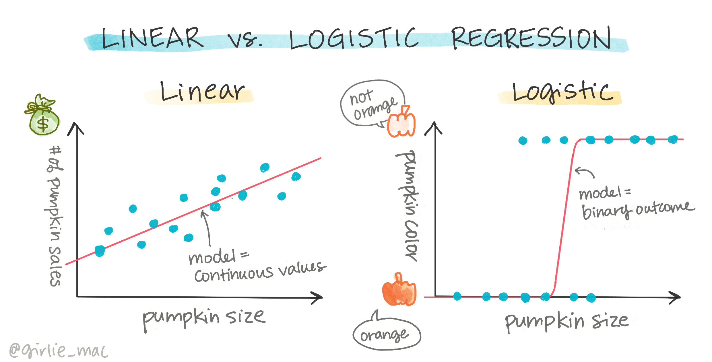
Logistic regression က Linear regression နဲ့ အရေးကြီးတဲ့ အချက်အချို့မှာ ကွဲပြားပါတယ်။

🎥 Logistic regression အကြောင်း အကျဉ်းချုပ်ဗီဒီယိုကို ကြည့်ရန် အထက်ပါပုံကို နှိပ်ပါ။

Binary classification

Logistic regression က Linear regression နဲ့ တူညီတဲ့ feature များ မပေးပါဘူး။ Logistic regression က binary အမျိုးအစား ("white or not white") ကို ခန့်မှန်းနိုင်သလို, Linear regression ကတော့ ဆက်လက်တိုးတက်နေတဲ့ အချက်အလက်များကို ခန့်မှန်းနိုင်ပါတယ်။ ဥပမာ - ဖရဲသီးရဲ့ မူလနေရာနဲ့ ခူးဆွတ်ချိန်အပေါ် မူတည်ပြီး ဈေးနှုန်းဘယ်လောက်တက်မလဲ ဆိုတာကို ခန့်မှန်းနိုင်ပါတယ်။

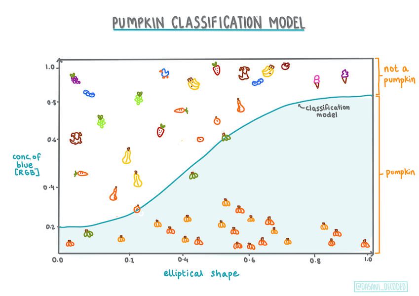
Infographic by Dasani Madipalli

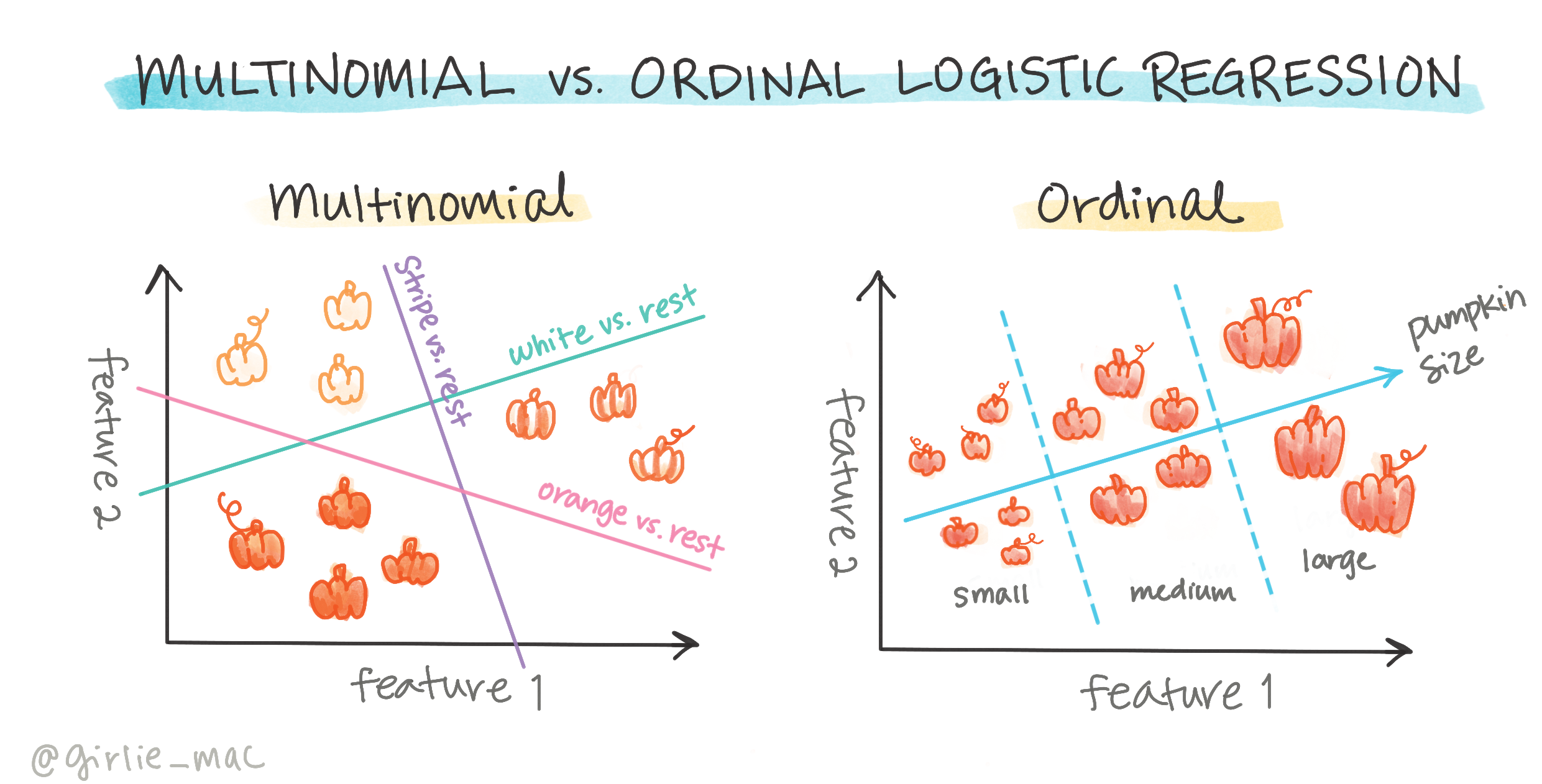
အခြား classification များ

Logistic regression ရဲ့ အခြားအမျိုးအစားများလည်း ရှိပါတယ်၊ Multinomial နဲ့ Ordinal အပါအဝင်:

Multinomial - အမျိုးအစားများစွာ ပါဝင်သောအခါ ("Orange, White, and Striped").
Ordinal - အမျိုးအစားများကို အစီအစဉ်အလိုက် စီရင်သောအခါ, ဥပမာ - ဖရဲသီးများကို အရွယ်အစား (mini, sm, med, lg, xl, xxl) အလိုက် စီရင်ခြင်း။

Variables များ correlation မလိုအပ်ပါ

Linear regression က correlation များရှိတဲ့ variables တွေကို ပိုကောင်းစွာ အလုပ်လုပ်နိုင်ပါတယ်။ Logistic regression ကတော့ ဆန့်ကျင်ဘက်ဖြစ်ပြီး - variables တွေ alignment မလိုအပ်ပါဘူး။ ဒါက correlation များအားနည်းတဲ့ ဒီဒေတာအတွက် အဆင်ပြေပါတယ်။

သန့်ရှင်းတဲ့ ဒေတာများ များများလိုအပ်ပါတယ်

Logistic regression က ဒေတာများ များများသုံးရင် ပိုမိုတိကျတဲ့ ရလဒ်တွေ ပေးနိုင်ပါတယ်။ ကျွန်တော်တို့ dataset က သေးငယ်တဲ့အတွက်, ဒီ task အတွက် အကောင်းဆုံးမဟုတ်ပါဘူး၊ ဒါကို သတိထားပါ။

🎥 Linear regression အတွက် ဒေတာကို ပြင်ဆင်ခြင်းအကြောင်း အကျဉ်းချုပ်ဗီဒီယိုကို ကြည့်ရန် အထက်ပါပုံကို နှိပ်ပါ။

✅ Logistic regression အတွက် သင့်လျော်တဲ့ ဒေတာအမျိုးအစားများကို စဉ်းစားပါ

လေ့ကျင့်ခန်း - ဒေတာကို tidy လုပ်ပါ

ပထမဦးဆုံး, null values တွေကို ဖယ်ရှားပြီး column အချို့ကိုသာ ရွေးချယ်ပါ:

အောက်ပါ code ကို ထည့်ပါ:


columns_to_select = ['City Name','Package','Variety', 'Origin','Item Size', 'Color']
pumpkins = full_pumpkins.loc[:, columns_to_select]

pumpkins.dropna(inplace=True)

သင့် dataframe အသစ်ကို အမြဲကြည့်ရှုနိုင်ပါတယ်:

pumpkins.info

Visualization - categorical plot

Starter notebook starter notebook ကို pumpkin data နဲ့ ပြန်တင်ပြီး, Color အပါအဝင် variables အချို့ကို ထိန်းသိမ်းထားတဲ့ dataset ကို သန့်စင်ပြီးဖြစ်ပါပြီ။ Notebook မှာ dataframe ကို visualized လုပ်ဖို့ Seaborn Seaborn ဆိုတဲ့ library အသစ်ကို အသုံးပြုပါမည်။

Seaborn က ဒေတာကို visualized လုပ်ဖို့ အဆင်ပြေတဲ့ နည်းလမ်းများ ပေးပါတယ်။ ဥပမာ - Variety နဲ့ Color တို့ရဲ့ distribution ကို categorical plot မှာ နှိုင်းယှဉ်နိုင်ပါတယ်။

Pumpkin data pumpkins ကို အသုံးပြုပြီး, ဖရဲသီး category (orange or white) တစ်ခုစီအတွက် အရောင် mapping ကို သတ်မှတ်ပြီး catplot function ကို အသုံးပြုပါ:
```
import seaborn as sns

palette = {
'ORANGE': 'orange',
'WHITE': 'wheat',
}

sns.catplot(
data=pumpkins, y="Variety", hue="Color", kind="count",
palette=palette,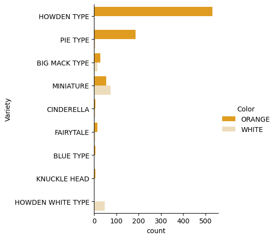 
)
```
ဒေတာကို ကြည့်ရှုခြင်းအားဖြင့်, Color data က Variety နဲ့ ဘယ်လိုဆက်စပ်နေသလဲဆိုတာကို တွေ့နိုင်ပါတယ်။

✅ ဒီ categorical plot ကို ကြည့်ပြီး, စိတ်ဝင်စားစရာ အခြေခံအချက်များကို စဉ်းစားပါ

Data pre-processing: feature and label encoding

Pumpkins dataset မှာ column အားလုံး string values ပါဝင်ပါတယ်။ Categorical data ကို လူတွေ အလွယ်တကူ နားလည်နိုင်ပေမယ့်, machine learning algorithms တွေကတော့ numbers နဲ့ ပိုကောင်းစွာ အလုပ်လုပ်နိုင်ပါတယ်။ ဒါကြောင့် encoding က data pre-processing အဆင့်မှာ အရေးကြီးတဲ့ အဆင့်ဖြစ်ပါတယ်။ ဒါက categorical data ကို numerical data အဖြစ် ပြောင်းနိုင်စေပြီး, အချက်အလက်မဆုံးရှုံးစေပါဘူး။ ကောင်းမွန်တဲ့ encoding က ကောင်းမွန်တဲ့ model တည်ဆောက်နိုင်စေပါတယ်။

Feature encoding အတွက် အဓိက encoder အမျိုးအစားနှစ်မျိုးရှိပါတယ်:

Ordinal encoder: Ordinal variables အတွက် သင့်လျော်ပါတယ်။ Ordinal variables ဆိုတာ logical ordering ရှိတဲ့ categorical variables ဖြစ်ပါတယ်။ ဥပမာ - dataset ရဲ့ Item Size column. Ordinal encoder က mapping တစ်ခု ဖန်တီးပြီး, category တစ်ခုစီကို column ရဲ့ အစီအစဉ်အလိုက် နံပါတ်တစ်ခုဖြင့် ကိုယ်စားပြုပါတယ်။
```
from sklearn.preprocessing import OrdinalEncoder

item_size_categories = [['sml', 'med', 'med-lge', 'lge', 'xlge', 'jbo', 'exjbo']]
ordinal_features = ['Item Size']
ordinal_encoder = OrdinalEncoder(categories=item_size_categories)
```
Categorical encoder: Nominal variables အတွက် သင့်လျော်ပါတယ်။ Nominal variables ဆိုတာ logical ordering မရှိတဲ့ categorical variables ဖြစ်ပါတယ်။ One-hot encoding ဖြစ်ပြီး, category တစ်ခုစီကို binary column ဖြင့် ကိုယ်စားပြုပါတယ်။ Encoded variable က ဖရဲသီးက အဲဒီ Variety ကိုယ်စားပြုရင် 1 ဖြစ်ပြီး, မဟုတ်ရင် 0 ဖြစ်ပါတယ်။
```
from sklearn.preprocessing import OneHotEncoder

categorical_features = ['City Name', 'Package', 'Variety', 'Origin']
categorical_encoder = OneHotEncoder(sparse_output=False)
```

ပြီးနောက်, ColumnTransformer ကို အသုံးပြုပြီး, encoder များစွာကို တစ်ခုတည်းသောအဆင့်အဖြစ် ပေါင်းစည်းပြီး သင့် columns များကို အကျိုးသက်ရောက်စေပါမည်။

    from sklearn.compose import ColumnTransformer
    
    ct = ColumnTransformer(transformers=[
        ('ord', ordinal_encoder, ordinal_features),
        ('cat', categorical_encoder, categorical_features)
        ])
    
    ct.set_output(transform='pandas')
    encoded_features = ct.fit_transform(pumpkins)

Label ကို encode လုပ်ဖို့, scikit-learn ရဲ့ LabelEncoder class ကို အသုံးပြုပါမည်။ LabelEncoder က labels တွေကို normalize လုပ်ပြီး, 0 နဲ့ n_classes-1 (ဒီမှာ 0 နဲ့ 1) အကြားရှိတဲ့ values တွေကိုသာ ပါဝင်စေပါတယ်။

    from sklearn.preprocessing import LabelEncoder

    label_encoder = LabelEncoder()
    encoded_label = label_encoder.fit_transform(pumpkins['Color'])

Features နဲ့ label ကို encode လုပ်ပြီးနောက်, encoded_pumpkins ဆိုတဲ့ dataframe အသစ်တစ်ခုအဖြစ် ပေါင်းစည်းနိုင်ပါတယ်။

    encoded_pumpkins = encoded_features.assign(Color=encoded_label)

✅ Item Size column အတွက် ordinal encoder ကို အသုံးပြုခြင်းရဲ့ အကျိုးကျေးဇူးများက ဘာတွေလဲ?

Variables များအကြား ဆက်နွယ်မှုများကို ချဉ်းကပ်ပါ

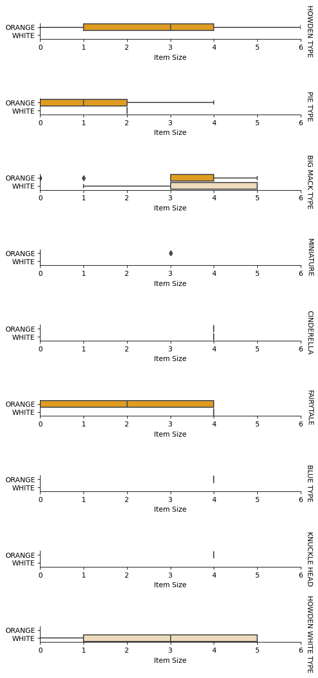
Data pre-processing ပြီးနောက်, features နဲ့ label အကြား ဆက်နွယ်မှုများကို ချဉ်းကပ်နိုင်ပါပြီ။ Model က features တွေကို အသုံးပြုပြီး label ကို ခန့်မှန်းနိုင်မယ့် အခြေအနေကို နားလည်ရန်, ဒေတာကို plot လုပ်ခြင်းက အကောင်းဆုံးနည်းလမ်းဖြစ်ပါတယ်။ Seaborn ရဲ့ catplot function ကို အသုံးပြုပြီး, Item Size, Variety နဲ့ Color တို့ရဲ့ ဆက်နွယ်မှုကို categorical plot မှာ visualized လုပ်ပါမည်။ Encoded Item Size column နဲ့ unencoded Variety column ကို အသုံးပြုပါမည်။

    palette = {
    'ORANGE': 'orange',
    'WHITE': 'wheat',
    }
    pumpkins['Item Size'] = encoded_pumpkins['ord__Item Size']

    g = sns.catplot(
        data=pumpkins,
        x="Item Size", y="Color", row='Variety',
        kind="box", orient="h",
        sharex=False, margin_titles=True,
        height=1.8, aspect=4, palette=palette,
    )
    g.set(xlabel="Item Size", ylabel="").set(xlim=(0,6))
    g.set_titles(row_template="{row_name}")

Swarm plot ကို အသုံးပြုပါ

Color က binary category (White or Not) ဖြစ်တဲ့အတွက်, 'a specialized approach to visualization' လိုအပ်ပါတယ်။ Category နဲ့ အခြား variables တွေကြား ဆက်နွယ်မှုကို visualized လုပ်ဖို့ အခြားနည်းလမ်းများလည်း ရှိပါတယ်။

Seaborn plots ကို အသုံးပြုပြီး, variables တွေကို side-by-side visualized လုပ်နိုင်ပါတယ်။

Values တွေ distribution ကို ပြသဖို့ 'swarm' plot ကို စမ်းသုံးပါ:

palette = {
0: 'orange',
1: 'wheat'
}
sns.swarmplot(x="Color", y="ord__Item Size", data=encoded_pumpkins, palette=palette)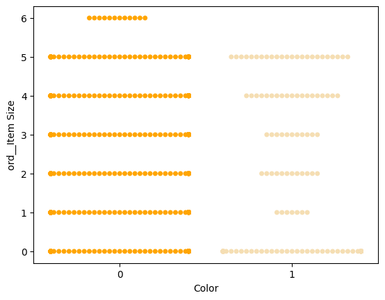

သတိထားပါ: အထက်ပါ code က warning တစ်ခု ဖြစ်စေနိုင်ပါတယ်၊ အကြောင်းကတော့ seaborn က datapoints များစွာကို swarm plot မှာ represent လုပ်ဖို့ မအောင်မြင်တာကြောင့် ဖြစ်ပါတယ်။ Marker size ကို 'size' parameter ဖြင့် လျှော့ချခြင်းက ဖြေရှင်းနည်းတစ်ခုဖြစ်နိုင်ပါတယ်။ သို့သော်, ဒါက plot ရဲ့ readability ကို ထိခိုက်စေနိုင်တာကို သတိထားပါ။

🧮 သင်္ချာကို ပြပါ

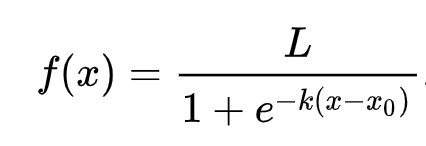
Logistic regression က 'maximum likelihood' concept ကို sigmoid functions အသုံးပြုပါတယ်။ 'Sigmoid Function' ဟာ plot မှာ 'S' ပုံစံရှိပါတယ်။ Value တစ်ခုကို 0 နဲ့ 1 အကြား map လုပ်ပါတယ်။ Curve ကို 'logistic curve' လို့လည်း ခေါ်ပါတယ်။ Formula က ဒီလိုပုံစံရှိပါတယ်:

Sigmoid ရဲ့ midpoint က x ရဲ့ 0 point မှာ ရှိပြီး, L က curve ရဲ့ အများဆုံး value ဖြစ်ပါတယ်။ k က curve ရဲ့ steepness ဖြစ်ပါတယ်။ Function ရဲ့ result က 0.5 ထက်ပိုရင်, label ကို binary choice ရဲ့ '1' class အဖြစ် assign လုပ်ပါမည်။ မဟုတ်ရင်, '0' အဖြစ် classify လုပ်ပါမည်။

Model ကို တည်ဆောက်ပါ

Binary classification တွေကို ရှာဖွေဖို့ model တစ်ခု တည်ဆောက်ခြင်းက Scikit-learn မှာ အလွယ်ကူပါတယ်။

🎥 Linear regression model တည်ဆောက်ခြင်းအကြောင်း အကျဉ်းချုပ်ဗီဒီယိုကို ကြည့်ရန် အထက်ပါပုံကို နှိပ်ပါ။

Classification model မှာ အသုံးပြုလိုတဲ့ variables တွေကို ရွေးချယ်ပြီး, train_test_split() ကို ခေါ်ပြီး training နဲ့ test sets ကို ခွဲပါ:

from sklearn.model_selection import train_test_split

X = encoded_pumpkins[encoded_pumpkins.columns.difference(['Color'])]
y = encoded_pumpkins['Color']

X_train, X_test, y_train, y_test = train_test_split(X, y, test_size=0.2, random_state=0)

Model ကို training data နဲ့ fit() ကို ခေါ်ပြီး train လုပ်ပါ၊ ရလဒ်ကို print လုပ်ပါ:

from sklearn.metrics import f1_score, classification_report 
from sklearn.linear_model import LogisticRegression

model = LogisticRegression()
model.fit(X_train, y_train)
predictions = model.predict(X_test)

print(classification_report(y_test, predictions))
print('Predicted labels: ', predictions)
print('F1-score: ', f1_score(y_test, predictions))

Model ရဲ့ scoreboard ကို ကြည့်ပါ။ ဒေတာ 1000 rows လောက်ပဲ ရှိတာကို တွေးမိရင်, အဆင်ပြေပါတယ်:

                   precision    recall  f1-score   support

                0       0.94      0.98      0.96       166
                1       0.85      0.67      0.75        33

    accuracy                                0.92       199
    macro avg           0.89      0.82      0.85       199
    weighted avg        0.92      0.92      0.92       199

    Predicted labels:  [0 0 0 0 0 0 0 0 0 0 0 0 0 0 0 0 0 0 0 0 1 0 0 1 0 0 0 0 0 0 0 0 1 0 0 0 0
    0 0 0 0 0 1 0 1 0 0 1 0 0 0 0 0 1 0 1 0 1 0 1 0 0 0 0 0 0 0 0 0 0 0 0 0 0
    1 0 0 0 0 0 0 0 1 0 0 0 0 0 0 0 1 0 0 0 0 0 0 0 0 1 0 1 0 0 0 0 0 0 0 1 0
    0 0 0 0 0 0 0 0 0 0 0 0 0 0 0 0 0 0 0 0 0 1 0 0 0 0 0 0 0 0 1 0 0 0 1 1 0
    0 0 0 0 1 0 0 0 0 0 1 0 0 0 0 0 0 0 0 0 0 0 0 0 0 0 0 0 0 0 0 0 0 0 0 0 1
    0 0 0 1 0 0 0 0 0 0 0 0 1 1]
    F1-score:  0.7457627118644068

Confusion matrix ဖြင့် ပိုမိုနားလည်မှုရရှိပါ

အထက်ပါ items တွေကို print လုပ်ပြီး, terms ရဲ့ scoreboard report ကို ရနိုင်ပါတယ်။ သို့သော်, model ကို ပိုမိုနားလည်စေရန်, confusion matrix ကို အသုံးပြုပါ။

🎓 'confusion matrix' (သို့မဟုတ် 'error matrix') က model ရဲ့ true vs. false positives နဲ့ negatives ကို table အနေနဲ့ ဖော်ပြပြီး, ခန့်မှန်းမှုရဲ့ တိကျမှုကို တိုင်းတာပါတယ်။

Confusion matrix ကို အသုံးပြုဖို့, confusion_matrix() ကို ခေါ်ပါ:
```
from sklearn.metrics import confusion_matrix
confusion_matrix(y_test, predictions)
```
Model ရဲ့ confusion matrix ကို ကြည့်ပါ:
```
array([[162,   4],
       [ 11,  22]])
```

Scikit-learn မှာ confusion matrices ရဲ့ Rows (axis 0) က actual labels ဖြစ်ပြီး, Columns (axis 1) က predicted labels ဖြစ်ပါတယ်။

	0	1
0	TN	FP

အကြောင်းအရာများနှင့် Precision နှင့် Recall တို့သည် Confusion Matrix နှင့် ဘယ်လိုဆက်စပ်နေသလဲ? အထက်တွင် ဖော်ပြထားသော Classification Report မှ Precision (0.85) နှင့် Recall (0.67) ကို ပြထားသည်။

Precision = tp / (tp + fp) = 22 / (22 + 4) = 0.8461538461538461

Recall = tp / (tp + fn) = 22 / (22 + 11) = 0.6666666666666666

✅ Q: Confusion Matrix အရ မော်ဒယ်က ဘယ်လိုလုပ်ဆောင်ခဲ့သလဲ?
A: မဆိုးပါဘူး၊ true negatives များစွာရှိပြီး false negatives အနည်းငယ်လည်းရှိပါတယ်။

Confusion Matrix မှ TP/TN နှင့် FP/FN mapping ကို အသုံးပြု၍ အရင်တွေ့ခဲ့သော အကြောင်းအရာများကို ပြန်လည်သုံးသပ်ကြမယ်။

🎓 Precision: TP/(TP + FP)
Retrieved ဖြစ်သော instances တွင် Relevant ဖြစ်သော instances ရဲ့ အချိုး (ဥပမာ- label များကို မှန်ကန်စွာ label လုပ်ထားသည်)

🎓 Recall: TP/(TP + FN)
Relevant ဖြစ်သော instances တွေကို Retrieved လုပ်ထားသော အချိုး (မှန်ကန်စွာ label လုပ်ထားခြင်းဖြစ်စေ၊ မဖြစ်စေ)

🎓 f1-score: (2 * precision * recall)/(precision + recall)
Precision နှင့် Recall ရဲ့ Weighted Average (အကောင်းဆုံး 1 ဖြစ်ပြီး အဆိုးဆုံး 0 ဖြစ်သည်)

🎓 Support:
Retrieved လုပ်ထားသော label တစ်ခုချင်းစီရဲ့ ဖြစ်ပေါ်မှုအရေအတွက်

🎓 Accuracy: (TP + TN)/(TP + TN + FP + FN)
Sample တစ်ခုအတွက် label များကို မှန်ကန်စွာ ခန့်မှန်းထားသော ရာခိုင်နှုန်း

🎓 Macro Avg:
Label များရဲ့ Imbalance ကို မထည့်သွင်းစဉ်းစားဘဲ Label တစ်ခုချင်းစီအတွက် Unweighted Mean Metrics တွေကို တွက်ချက်ထားခြင်း

🎓 Weighted Avg:
Label များရဲ့ Imbalance ကို Support (label တစ်ခုချင်းစီရဲ့ true instances အရေအတွက်) ဖြင့် weighting လုပ်ပြီး Mean Metrics တွေကို တွက်ချက်ထားခြင်း

✅ Q: False negatives အရေအတွက်ကို လျှော့ချချင်ရင် မော်ဒယ်ရဲ့ ဘယ် Metric ကို အဓိကကြည့်သင့်သလဲ?

မော်ဒယ်ရဲ့ ROC Curve ကို Visualize လုပ်ပါ

🎥 အထက်ပါပုံကို Click လုပ်ပြီး ROC Curves အကြောင်း ရှင်းလင်းထားသော ဗီဒီယိုကို ကြည့်ပါ

"ROC" Curve ကို ကြည့်ရှုရန် Visualization တစ်ခုကို ပြုလုပ်ကြမယ်။

from sklearn.metrics import roc_curve, roc_auc_score
import matplotlib
import matplotlib.pyplot as plt
%matplotlib inline

y_scores = model.predict_proba(X_test)
fpr, tpr, thresholds = roc_curve(y_test, y_scores[:,1])

fig = plt.figure(figsize=(6, 6))
plt.plot([0, 1], [0, 1], 'k--')
plt.plot(fpr, tpr)
plt.xlabel('False Positive Rate')
plt.ylabel('True Positive Rate')
plt.title('ROC Curve')
plt.show()

Matplotlib ကို အသုံးပြု၍ မော်ဒယ်ရဲ့ Receiving Operating Characteristic (ROC) ကို Plot လုပ်ပါ။ ROC curves ကို Classifier ရဲ့ True vs. False Positives output ကို ကြည့်ရှုရန် အများအားဖြင့် အသုံးပြုသည်။ "ROC curves တွင် Y axis တွင် True Positive Rate ကို feature လုပ်ပြီး X axis တွင် False Positive Rate ကို feature လုပ်သည်။" Curve ရဲ့ steepness နှင့် Midpoint Line နှင့် Curve အကြားရှိနေသော နေရာသည် အရေးကြီးသည်။ Curve က မြန်မြန် Heading Up လုပ်ပြီး Line အပေါ်ကို ရောက်သင့်သည်။ ကျွန်ုပ်တို့ရဲ့ မော်ဒယ်တွင် False Positives များစွာရှိပြီး Line က Heading Up လုပ်ပြီး အပေါ်ကို ရောက်သွားသည်။

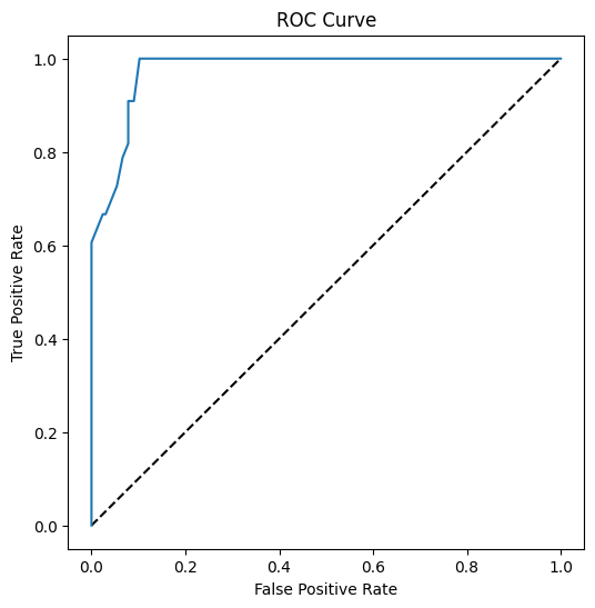
နောက်ဆုံးတွင် Scikit-learn ရဲ့ roc_auc_score API ကို အသုံးပြု၍ 'Area Under the Curve' (AUC) ကို တွက်ချက်ပါ။

auc = roc_auc_score(y_test,y_scores[:,1])
print(auc)

ရလဒ်မှာ 0.9749908725812341 ဖြစ်သည်။ AUC သည် 0 မှ 1 အထိ ရှိနိုင်ပြီး Prediction များကို 100% မှန်ကန်စွာ ခန့်မှန်းနိုင်သော မော်ဒယ်သည် AUC 1 ရှိမည်။ ဒီအခါမှာတော့ မော်ဒယ်က တော်တော်လေးကောင်းပါတယ်။

အနာဂတ် Classifications သင်ခန်းစာများတွင် မော်ဒယ်ရဲ့ Score များကို တိုးတက်အောင် Iteration လုပ်နည်းကို သင်ယူရမည်။ ဒါပေမယ့် အခုအချိန်မှာ Congratulations! Regression သင်ခန်းစာများကို ပြီးမြောက်စွာ လုပ်ဆောင်နိုင်ပါပြီ!

🚀Challenge

Logistic Regression အကြောင်းမှာ သင်ယူစရာများစွာ ရှိနေဆဲပါ။ သို့သော် အကောင်းဆုံး သင်ယူနည်းက စမ်းသပ်ခြင်းဖြစ်သည်။ ဒီအမျိုးအစား Analysis အတွက် သင့်လျော်သော Dataset တစ်ခုကို ရှာဖွေပြီး မော်ဒယ်တစ်ခုကို တည်ဆောက်ပါ။ သင်ဘာတွေ သင်ယူရမလဲ? tip: Kaggle မှ စိတ်ဝင်စားဖွယ် Dataset များကို စမ်းကြည့်ပါ။

Post-lecture quiz

Review & Self Study

Stanford မှ ဒီစာတမ်း ရဲ့ ပထမပိုင်းစာမျက်နှာများကို ဖတ်ပါ။ Logistic Regression ရဲ့ လက်တွေ့အသုံးချမှုများအကြောင်းတွင် စဉ်းစားပါ။ ကျွန်ုပ်တို့ သင်ယူခဲ့သော Regression အမျိုးအစားများအနက် ဘယ်အမျိုးအစားက သင့်လျော်မလဲဆိုတာကို စဉ်းစားပါ။

Assignment

Retrying this regression

ဝက်ဘ်ဆိုက်မှတ်ချက်:
ဤစာရွက်စာတမ်းကို AI ဘာသာပြန်ဝန်ဆောင်မှု Co-op Translator ကို အသုံးပြု၍ ဘာသာပြန်ထားပါသည်။ ကျွန်ုပ်တို့သည် တိကျမှန်ကန်မှုအတွက် ကြိုးစားနေပါသော်လည်း၊ အလိုအလျောက်ဘာသာပြန်ဆိုမှုများတွင် အမှားများ သို့မဟုတ် မမှန်ကန်မှုများ ပါဝင်နိုင်သည်ကို ကျေးဇူးပြု၍ သတိပြုပါ။ မူရင်းစာရွက်စာတမ်းကို ၎င်း၏ မူလဘာသာစကားဖြင့် အာဏာတည်သောရင်းမြစ်အဖြစ် သတ်မှတ်ရန် လိုအပ်ပါသည်။ အရေးကြီးသော အချက်အလက်များအတွက် လူကောင်းမွန်သော ပရော်ဖက်ရှင်နယ်ဘာသာပြန်ဝန်ဆောင်မှုကို အကြံပြုပါသည်။ ဤဘာသာပြန်ကို အသုံးပြုခြင်းမှ ဖြစ်ပေါ်လာသော နားလည်မှုမှားများ သို့မဟုတ် အဓိပ္ပာယ်မှားများအတွက် ကျွန်ုပ်တို့သည် တာဝန်မယူပါ။

35 KiB Raw Permalink Blame History