18 KiB

Raw Permalink Blame History Unescape Escape

小车杆平衡

在前一课中我们解决的问题看起来像是一个玩具问题，似乎并不适用于实际场景。但事实并非如此，因为许多现实世界的问题也有类似的场景，包括下棋或围棋。它们是相似的，因为我们也有一个带有给定规则的棋盘和一个离散状态。

课前测验

介绍

在本课中，我们将把Q学习的相同原理应用到一个连续状态的问题上，即由一个或多个实数给定的状态。我们将处理以下问题：

问题：如果彼得想要逃离狼，他需要能够更快地移动。我们将看看彼得如何学习滑冰，特别是如何通过Q学习保持平衡。

彼得和他的朋友们想出妙招逃离狼！图片来自 Jen Looper

我们将使用一种称为小车杆问题的简化平衡版本。在小车杆世界中，我们有一个可以左右移动的水平滑块，目标是让垂直杆在滑块上保持平衡。

先决条件

在本课中，我们将使用一个名为OpenAI Gym的库来模拟不同的环境。你可以在本地运行本课的代码（例如在Visual Studio Code中），在这种情况下，模拟将会在一个新窗口中打开。当在线运行代码时，你可能需要对代码进行一些调整，如这里所述。

OpenAI Gym

在前一课中，游戏的规则和状态由我们自己定义的Board类给出。这里我们将使用一个特殊的模拟环境，它将模拟平衡杆背后的物理现象。训练强化学习算法最流行的模拟环境之一是由OpenAI维护的Gym。通过使用这个gym，我们可以创建从小车杆模拟到Atari游戏的不同环境。

注意：你可以在这里查看OpenAI Gym提供的其他环境。

首先，让我们安装gym并导入所需的库（代码块1）：

import sys
!{sys.executable} -m pip install gym 

import gym
import matplotlib.pyplot as plt
import numpy as np
import random

练习 - 初始化一个小车杆环境

要处理小车杆平衡问题，我们需要初始化相应的环境。每个环境都与一个：

观察空间相关，定义我们从环境中接收的信息结构。对于小车杆问题，我们接收杆的位置、速度和其他一些值。
动作空间相关，定义可能的动作。在我们的案例中，动作空间是离散的，由两个动作组成 - 左和右。（代码块2）

要初始化，请输入以下代码：

env = gym.make("CartPole-v1")
print(env.action_space)
print(env.observation_space)
print(env.action_space.sample())

要查看环境如何工作，让我们运行一个100步的简短模拟。在每一步，我们提供一个要采取的动作 - 在此模拟中，我们只是随机选择一个来自action_space的动作。

运行下面的代码，看看会导致什么结果。

✅ 记住，最好在本地Python安装中运行此代码！（代码块3）
```
env.reset()

for i in range(100):
   env.render()
   env.step(env.action_space.sample())
env.close()
```
你应该会看到类似这样的图像：

在模拟过程中，我们需要获取观察值以决定如何行动。事实上，step函数返回当前的观察值、奖励函数和一个表示是否继续模拟的完成标志：（代码块4）

env.reset()

done = False
while not done:
   env.render()
   obs, rew, done, info = env.step(env.action_space.sample())
   print(f"{obs} -> {rew}")
env.close()

你将在笔记本输出中看到类似这样的内容：

[ 0.03403272 -0.24301182  0.02669811  0.2895829 ] -> 1.0
[ 0.02917248 -0.04828055  0.03248977  0.00543839] -> 1.0
[ 0.02820687  0.14636075  0.03259854 -0.27681916] -> 1.0
[ 0.03113408  0.34100283  0.02706215 -0.55904489] -> 1.0
[ 0.03795414  0.53573468  0.01588125 -0.84308041] -> 1.0
...
[ 0.17299878  0.15868546 -0.20754175 -0.55975453] -> 1.0
[ 0.17617249  0.35602306 -0.21873684 -0.90998894] -> 1.0

在模拟的每一步返回的观察向量包含以下值：

小车的位置
小车的速度
杆的角度
杆的旋转速率

获取这些数字的最小值和最大值：（代码块5）
```
print(env.observation_space.low)
print(env.observation_space.high)
```
你可能还会注意到，每一步模拟的奖励值总是1。这是因为我们的目标是尽可能长时间地生存，即尽可能长时间地保持杆在合理的垂直位置。

✅ 实际上，如果我们能在100次连续试验中平均获得195的奖励，小车杆模拟就被认为是解决了。

状态离散化

在Q学习中，我们需要构建Q表，定义在每个状态下该做什么。为了能够做到这一点，我们需要状态是离散的，更准确地说，它应该包含有限数量的离散值。因此，我们需要以某种方式离散化我们的观察值，将它们映射到有限的状态集合。

有几种方法可以做到这一点：

划分为箱子。如果我们知道某个值的区间，我们可以将该区间划分为多个箱子，然后用它所属的箱子编号替换该值。这可以使用numpy的digitize方法来完成。在这种情况下，我们将准确知道状态的大小，因为它将取决于我们为数字化选择的箱子数量。

✅ 我们可以使用线性插值将值带到某个有限区间（例如，从-20到20），然后通过四舍五入将数字转换为整数。这给了我们对状态大小的控制稍微少一些，特别是如果我们不知道输入值的确切范围。例如，在我们的例子中，4个值中的2个没有上/下限，这可能导致无限数量的状态。

在我们的例子中，我们将使用第二种方法。正如你可能稍后注意到的，尽管没有明确的上/下限，这些值很少会取到某些有限区间之外的值，因此那些具有极端值的状态将非常罕见。

这是一个函数，它将从我们的模型中获取观察值并生成一个包含4个整数值的元组：（代码块6）
```
def discretize(x):
    return tuple((x/np.array([0.25, 0.25, 0.01, 0.1])).astype(np.int))
```

让我们还探索另一种使用箱子的离散化方法：（代码块7）

def create_bins(i,num):
    return np.arange(num+1)*(i[1]-i[0])/num+i[0]

print("Sample bins for interval (-5,5) with 10 bins\n",create_bins((-5,5),10))

ints = [(-5,5),(-2,2),(-0.5,0.5),(-2,2)] # intervals of values for each parameter
nbins = [20,20,10,10] # number of bins for each parameter
bins = [create_bins(ints[i],nbins[i]) for i in range(4)]

def discretize_bins(x):
    return tuple(np.digitize(x[i],bins[i]) for i in range(4))

现在让我们运行一个简短的模拟并观察这些离散的环境值。随意尝试discretize and discretize_bins，看看是否有差异。

✅ discretize_bins返回箱子编号，这是从0开始的。因此，对于接近0的输入变量值，它返回区间中间的数字（10）。在discretize中，我们不关心输出值的范围，允许它们为负，因此状态值没有偏移，0对应于0。（代码块8）
```
env.reset()

done = False
while not done:
   #env.render()
   obs, rew, done, info = env.step(env.action_space.sample())
   #print(discretize_bins(obs))
   print(discretize(obs))
env.close()
```
✅ 如果你想查看环境的执行情况，请取消注释以env.render开头的行。否则，你可以在后台执行它，这样更快。在我们的Q学习过程中，我们将使用这种“隐形”执行。

Q表结构

在前一课中，状态是从0到8的简单数对，因此用形状为8x8x2的numpy张量表示Q表是方便的。如果我们使用箱子离散化，状态向量的大小也是已知的，所以我们可以使用相同的方法，用形状为20x20x10x10x2的数组表示状态（这里2是动作空间的维度，前面的维度对应于我们为观察空间中的每个参数选择的箱子数量）。

然而，有时观察空间的确切维度是不知道的。在discretize函数的情况下，我们可能永远无法确定我们的状态是否保持在某些限制内，因为某些原始值没有限制。因此，我们将使用一种稍微不同的方法，用字典表示Q表。

使用对*(state,action)*作为字典键，值对应于Q表条目值。（代码块9）
```
Q = {}
actions = (0,1)

def qvalues(state):
    return [Q.get((state,a),0) for a in actions]
```
这里我们还定义了一个函数qvalues()，它返回给定状态对应于所有可能动作的Q表值列表。如果Q表中没有该条目，我们将返回0作为默认值。

开始Q学习

现在我们准备教彼得保持平衡了！

首先，让我们设置一些超参数：（代码块10）
```
# hyperparameters
alpha = 0.3
gamma = 0.9
epsilon = 0.90
```
这里，alpha is the learning rate that defines to which extent we should adjust the current values of Q-Table at each step. In the previous lesson we started with 1, and then decreased alpha to lower values during training. In this example we will keep it constant just for simplicity, and you can experiment with adjusting alpha values later.

gamma is the discount factor that shows to which extent we should prioritize future reward over current reward.

epsilon is the exploration/exploitation factor that determines whether we should prefer exploration to exploitation or vice versa. In our algorithm, we will in epsilon percent of the cases select the next action according to Q-Table values, and in the remaining number of cases we will execute a random action. This will allow us to explore areas of the search space that we have never seen before.

✅ In terms of balancing - choosing random action (exploration) would act as a random punch in the wrong direction, and the pole would have to learn how to recover the balance from those "mistakes"

Improve the algorithm

We can also make two improvements to our algorithm from the previous lesson:

Calculate average cumulative reward, over a number of simulations. We will print the progress each 5000 iterations, and we will average out our cumulative reward over that period of time. It means that if we get more than 195 point - we can consider the problem solved, with even higher quality than required.
Calculate maximum average cumulative result, Qmax, and we will store the Q-Table corresponding to that result. When you run the training you will notice that sometimes the average cumulative result starts to drop, and we want to keep the values of Q-Table that correspond to the best model observed during training.

Collect all cumulative rewards at each simulation at rewards向量以便进一步绘图。（代码块11）

def probs(v,eps=1e-4):
    v = v-v.min()+eps
    v = v/v.sum()
    return v

Qmax = 0
cum_rewards = []
rewards = []
for epoch in range(100000):
    obs = env.reset()
    done = False
    cum_reward=0
    # == do the simulation ==
    while not done:
        s = discretize(obs)
        if random.random()<epsilon:
            # exploitation - chose the action according to Q-Table probabilities
            v = probs(np.array(qvalues(s)))
            a = random.choices(actions,weights=v)[0]
        else:
            # exploration - randomly chose the action
            a = np.random.randint(env.action_space.n)

        obs, rew, done, info = env.step(a)
        cum_reward+=rew
        ns = discretize(obs)
        Q[(s,a)] = (1 - alpha) * Q.get((s,a),0) + alpha * (rew + gamma * max(qvalues(ns)))
    cum_rewards.append(cum_reward)
    rewards.append(cum_reward)
    # == Periodically print results and calculate average reward ==
    if epoch%5000==0:
        print(f"{epoch}: {np.average(cum_rewards)}, alpha={alpha}, epsilon={epsilon}")
        if np.average(cum_rewards) > Qmax:
            Qmax = np.average(cum_rewards)
            Qbest = Q
        cum_rewards=[]

你可能从这些结果中注意到：

接近我们的目标。我们非常接近实现目标，即在100+次连续运行模拟中获得195的累计奖励，或者我们实际上已经实现了！即使我们得到较小的数字，我们也不知道，因为我们平均超过5000次运行，而正式标准仅需要100次运行。
奖励开始下降。有时奖励开始下降，这意味着我们可能用使情况变得更糟的新值“破坏”了Q表中已经学习到的值。

如果我们绘制训练进度，这一观察结果会更加明显。

绘制训练进度

在训练过程中，我们已经将每次迭代的累计奖励值收集到rewards向量中。以下是我们将其与迭代次数一起绘制时的样子：

plt.plot(rewards)

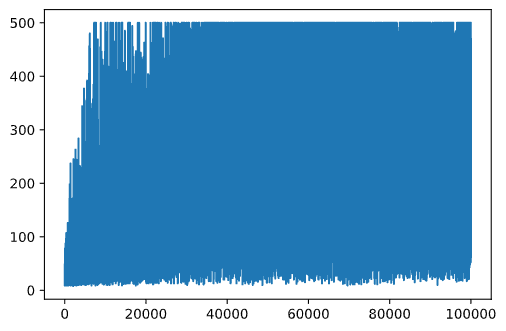
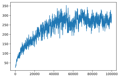
从这个图表中，我们无法判断任何事情，因为由于随机训练过程的性质，训练会话的长度变化很大。为了使这个图表更有意义，我们可以计算一系列实验的移动平均值，比如100。这可以方便地使用np.convolve完成：（代码块12）

def running_average(x,window):
    return np.convolve(x,np.ones(window)/window,mode='valid')

plt.plot(running_average(rewards,100))

调整超参数

为了使学习更加稳定，有必要在训练过程中调整一些超参数。特别是：

对于学习率，alpha, we may start with values close to 1, and then keep decreasing the parameter. With time, we will be getting good probability values in the Q-Table, and thus we should be adjusting them slightly, and not overwriting completely with new values.
Increase epsilon. We may want to increase the epsilon slowly, in order to explore less and exploit more. It probably makes sense to start with lower value of epsilon，并上升到几乎1。

任务1：尝试调整超参数值，看看是否能获得更高的累计奖励。你能达到195以上吗？

任务2：要正式解决这个问题，你需要在100次连续运行中获得195的平均奖励。在训练过程中测量这一点，并确保你已经正式解决了这个问题！

查看结果

实际上看到训练模型的行为会很有趣。让我们运行模拟，并按照训练期间的相同动作选择策略，根据Q表中的概率分布进行采样：（代码块13）

obs = env.reset()
done = False
while not done:
   s = discretize(obs)
   env.render()
   v = probs(np.array(qvalues(s)))
   a = random.choices(actions,weights=v)[0]
   obs,_,done,_ = env.step(a)
env.close()

你应该会看到类似这样的图像：

🚀挑战

任务3：这里，我们使用的是Q表的最终副本，这可能不是最好的。记住我们已经将表现最好的Q表存储在Qbest variable! Try the same example with the best-performing Q-Table by copying Qbest over to Q and see if you notice the difference.

Task 4: Here we were not selecting the best action on each step, but rather sampling with corresponding probability distribution. Would it make more sense to always select the best action, with the highest Q-Table value? This can be done by using np.argmax函数来找到对应于最高Q表值的动作编号。实现这一策略，看看它是否改善了平衡。

课后测验

作业

训练一辆山地车

结论

我们现在已经学会了如何通过提供定义游戏期望状态的奖励函数，并给他们机会智能地探索搜索空间，来训练智能体以取得良好的结果。我们已经成功地在离散和连续环境中应用了Q学习算法，但动作仍然是离散的。

重要的是还要研究动作状态也是连续的情况，以及观察空间更复杂的情况，例如来自Atari游戏屏幕的图像。在这些问题中，我们通常需要使用更强大的机器学习技术，例如神经网络，以取得良好的结果。这些更高级的话题是我们即将到来的更高级AI课程的主题。

免责声明：本文档是使用基于机器的人工智能翻译服务翻译的。尽管我们努力确保准确性，但请注意，自动翻译可能包含错误或不准确之处。应将原文档的母语版本视为权威来源。对于关键信息，建议进行专业的人工翻译。我们不对使用此翻译所产生的任何误解或误释承担责任。

18 KiB Raw Permalink Blame History Unescape Escape