14 KiB
美食分类器 1
在本课中,你将使用上节课保存的数据集,这些数据是关于美食的平衡、干净的数据。
你将使用这个数据集与各种分类器一起工作,根据一组食材预测给定的国家美食。在此过程中,你将了解一些算法如何被用来完成分类任务。
课前测验
准备工作
假设你已经完成了第一课,确保在根目录 /data 文件夹中存在一个 cleaned_cuisines.csv 文件,以供这四节课使用。
练习 - 预测国家美食
-
在本课的 notebook.ipynb 文件夹中,导入该文件和 Pandas 库:
import pandas as pd
cuisines_df = pd.read_csv("../data/cleaned_cuisines.csv")
cuisines_df.head()
数据看起来是这样的:
| Unnamed: 0 | cuisine | almond | angelica | anise | anise_seed | apple | apple_brandy | apricot | armagnac | ... | whiskey | white_bread | white_wine | whole_grain_wheat_flour | wine | wood | yam | yeast | yogurt | zucchini | |
|---|---|---|---|---|---|---|---|---|---|---|---|---|---|---|---|---|---|---|---|---|---|
| 0 | 0 | indian | 0 | 0 | 0 | 0 | 0 | 0 | 0 | 0 | ... | 0 | 0 | 0 | 0 | 0 | 0 | 0 | 0 | 0 | 0 |
| 1 | 1 | indian | 1 | 0 | 0 | 0 | 0 | 0 | 0 | 0 | ... | 0 | 0 | 0 | 0 | 0 | 0 | 0 | 0 | 0 | 0 |
| 2 | 2 | indian | 0 | 0 | 0 | 0 | 0 | 0 | 0 | 0 | ... | 0 | 0 | 0 | 0 | 0 | 0 | 0 | 0 | 0 | 0 |
| 3 | 3 | indian | 0 | 0 | 0 | 0 | 0 | 0 | 0 | 0 | ... | 0 | 0 | 0 | 0 | 0 | 0 | 0 | 0 | 0 | 0 |
| 4 | 4 | indian | 0 | 0 | 0 | 0 | 0 | 0 | 0 | 0 | ... | 0 | 0 | 0 | 0 | 0 | 0 | 0 | 0 | 1 | 0 |
-
现在,导入更多的库:
from sklearn.linear_model import LogisticRegression from sklearn.model_selection import train_test_split, cross_val_score from sklearn.metrics import accuracy_score,precision_score,confusion_matrix,classification_report, precision_recall_curve from sklearn.svm import SVC import numpy as np -
将 X 和 y 坐标分成两个用于训练的数据框架。
cuisine可以作为标签数据框:cuisines_label_df = cuisines_df['cuisine'] cuisines_label_df.head()它看起来是这样的:
0 indian 1 indian 2 indian 3 indian 4 indian Name: cuisine, dtype: object -
删除
Unnamed: 0column and thecuisinecolumn, callingdrop()列。将剩余的数据保存为可训练的特征:cuisines_feature_df = cuisines_df.drop(['Unnamed: 0', 'cuisine'], axis=1) cuisines_feature_df.head()你的特征看起来是这样的:
| almond | angelica | anise | anise_seed | apple | apple_brandy | apricot | armagnac | artemisia | artichoke | ... | whiskey | white_bread | white_wine | whole_grain_wheat_flour | wine | wood | yam | yeast | yogurt | zucchini | |
|---|---|---|---|---|---|---|---|---|---|---|---|---|---|---|---|---|---|---|---|---|---|
| 0 | 0 | 0 | 0 | 0 | 0 | 0 | 0 | 0 | 0 | 0 | ... | 0 | 0 | 0 | 0 | 0 | 0 | 0 | 0 | 0 | 0 |
| 1 | 1 | 0 | 0 | 0 | 0 | 0 | 0 | 0 | 0 | 0 | ... | 0 | 0 | 0 | 0 | 0 | 0 | 0 | 0 | 0 | 0 |
| 2 | 0 | 0 | 0 | 0 | 0 | 0 | 0 | 0 | 0 | 0 | ... | 0 | 0 | 0 | 0 | 0 | 0 | 0 | 0 | 0 | 0 |
| 3 | 0 | 0 | 0 | 0 | 0 | 0 | 0 | 0 | 0 | 0 | ... | 0 | 0 | 0 | 0 | 0 | 0 | 0 | 0 | 0 | 0 |
| 4 | 0 | 0 | 0 | 0 | 0 | 0 | 0 | 0 | 0 | 0 | ... | 0 | 0 | 0 | 0 | 0 | 0 | 0 | 0 | 1 | 0 |
现在你已经准备好训练你的模型了!
选择你的分类器
现在你的数据已经清理干净并准备好进行训练,你需要决定使用哪种算法来完成这项任务。
Scikit-learn 将分类归为监督学习,在这个类别中你会发现很多分类方法。 种类繁多,乍一看可能会让人眼花缭乱。以下方法都包含分类技术:
- 线性模型
- 支持向量机
- 随机梯度下降
- 最近邻
- 高斯过程
- 决策树
- 集成方法(投票分类器)
- 多类和多输出算法(多类和多标签分类,多类-多输出分类)
你也可以使用神经网络来分类数据,但这超出了本课的范围。
选择哪个分类器?
那么,你应该选择哪个分类器呢?通常,运行多个分类器并寻找一个好的结果是一种测试方法。Scikit-learn 提供了一个并排比较的创建数据集,比较了 KNeighbors、SVC 两种方式、GaussianProcessClassifier、DecisionTreeClassifier、RandomForestClassifier、MLPClassifier、AdaBoostClassifier、GaussianNB 和 QuadraticDiscrinationAnalysis,展示了结果的可视化:
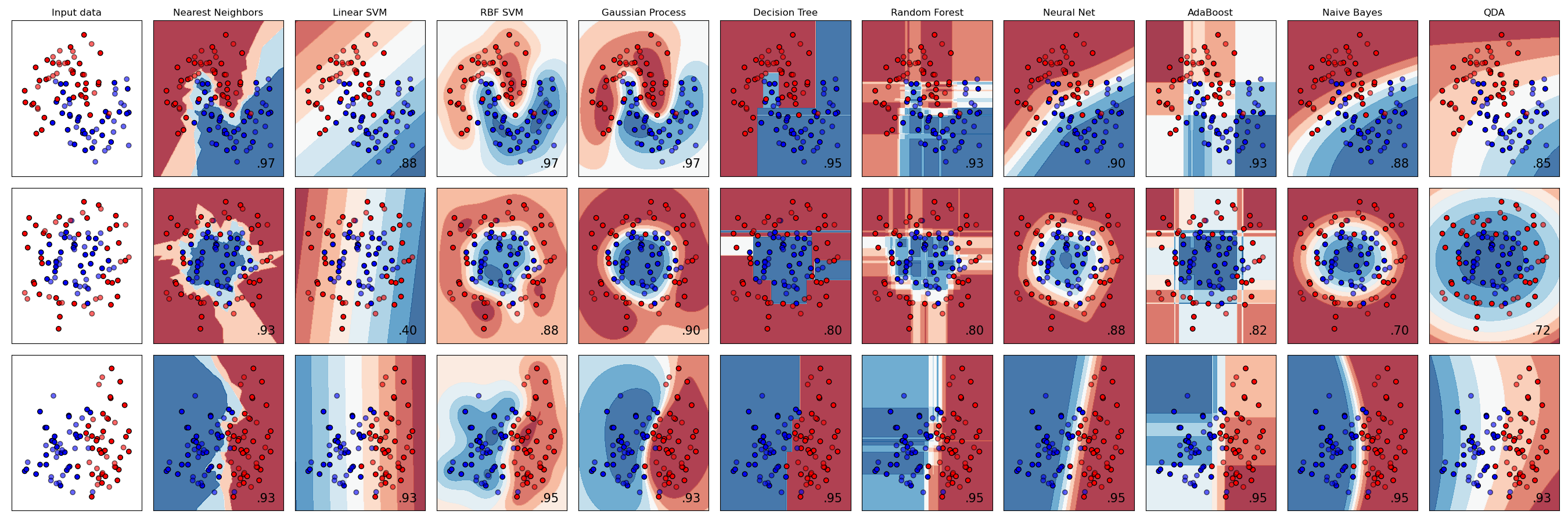
图表来自 Scikit-learn 的文档
AutoML 通过在云中运行这些比较,允许你选择最适合你数据的算法,巧妙地解决了这个问题。试试这里
更好的方法
比盲目猜测更好的方法是遵循这个可下载的机器学习速查表上的想法。在这里,我们发现,对于我们的多类问题,我们有一些选择:
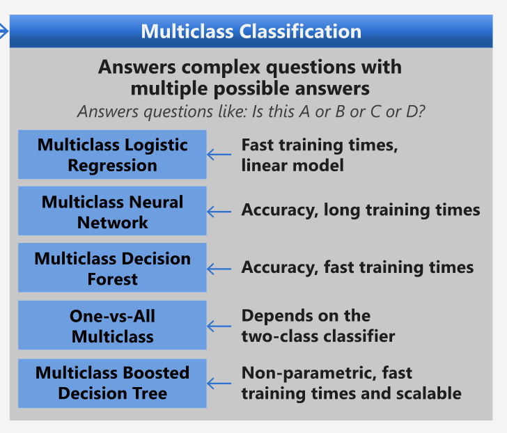
微软算法速查表的一部分,详细介绍了多类分类选项
✅ 下载这个速查表,打印出来,挂在墙上!
推理
让我们看看能否根据我们面临的限制推理出不同的方法:
- 神经网络太重了。考虑到我们的数据集干净但很少,并且我们是通过笔记本本地运行训练,神经网络对于这个任务来说太重了。
- 没有两类分类器。我们不使用两类分类器,因此排除了 one-vs-all。
- 决策树或逻辑回归可能有效。决策树可能有效,或者多类数据的逻辑回归。
- 多类增强决策树解决不同的问题。多类增强决策树最适合非参数任务,例如设计用于构建排名的任务,因此对我们没有用。
使用 Scikit-learn
我们将使用 Scikit-learn 来分析我们的数据。然而,在 Scikit-learn 中有许多方法可以使用逻辑回归。看看需要传递的参数。
本质上有两个重要参数 - multi_class and solver - that we need to specify, when we ask Scikit-learn to perform a logistic regression. The multi_class value applies a certain behavior. The value of the solver is what algorithm to use. Not all solvers can be paired with all multi_class values.
According to the docs, in the multiclass case, the training algorithm:
- Uses the one-vs-rest (OvR) scheme, if the
multi_classoption is set toovr - Uses the cross-entropy loss, if the
multi_classoption is set tomultinomial. (Currently themultinomialoption is supported only by the ‘lbfgs’, ‘sag’, ‘saga’ and ‘newton-cg’ solvers.)"
🎓 The 'scheme' here can either be 'ovr' (one-vs-rest) or 'multinomial'. Since logistic regression is really designed to support binary classification, these schemes allow it to better handle multiclass classification tasks. source
🎓 The 'solver' is defined as "the algorithm to use in the optimization problem". source.
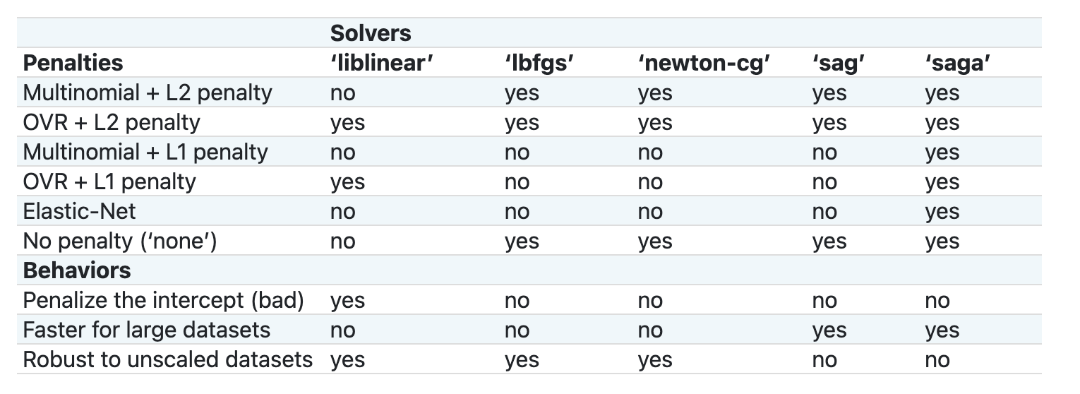
Scikit-learn offers this table to explain how solvers handle different challenges presented by different kinds of data structures:
Exercise - split the data
We can focus on logistic regression for our first training trial since you recently learned about the latter in a previous lesson.
Split your data into training and testing groups by calling train_test_split():
X_train, X_test, y_train, y_test = train_test_split(cuisines_feature_df, cuisines_label_df, test_size=0.3)
练习 - 应用逻辑回归
由于你使用的是多类情况,你需要选择什么 方案 和设置什么 求解器。使用 LogisticRegression 的多类设置和 liblinear 求解器进行训练。
-
创建一个多类设置为
ovrand the solver set toliblinear的逻辑回归:lr = LogisticRegression(multi_class='ovr',solver='liblinear') model = lr.fit(X_train, np.ravel(y_train)) accuracy = model.score(X_test, y_test) print ("Accuracy is {}".format(accuracy))✅ 尝试一个不同的求解器,例如
lbfgs, which is often set as defaultNote, use Pandas
ravel函数在需要时展平你的数据。准确率超过 80%,效果很好!
-
你可以通过测试一行数据(#50)来看到这个模型的实际效果:
print(f'ingredients: {X_test.iloc[50][X_test.iloc[50]!=0].keys()}')
print(f'cuisine: {y_test.iloc[50]}')
结果打印出来:
ingredients: Index(['cilantro', 'onion', 'pea', 'potato', 'tomato', 'vegetable_oil'], dtype='object')
cuisine: indian
✅ 尝试一个不同的行号并检查结果
-
更深入地了解,你可以检查这个预测的准确性:
test= X_test.iloc[50].values.reshape(-1, 1).T
proba = model.predict_proba(test)
classes = model.classes_
resultdf = pd.DataFrame(data=proba, columns=classes)

topPrediction = resultdf.T.sort_values(by=[0], ascending = [False])
topPrediction.head()
结果打印出来 - 印度菜是最好的猜测,概率很高:
0 indian 0.715851 chinese 0.229475 japanese 0.029763 korean 0.017277 thai 0.007634 ✅ 你能解释为什么模型非常确定这是印度菜吗?
-
通过打印分类报告,获取更多细节,就像在回归课程中所做的那样:
y_pred = model.predict(X_test)
print(classification_report(y_test,y_pred))
precision recall f1-score support chinese 0.73 0.71 0.72 229 indian 0.91 0.93 0.92 254 japanese 0.70 0.75 0.72 220 korean 0.86 0.76 0.81 242 thai 0.79 0.85 0.82 254 accuracy 0.80 1199 macro avg 0.80 0.80 0.80 1199 weighted avg 0.80 0.80 0.80 1199
🚀挑战
在本课中,你使用清理后的数据构建了一个机器学习模型,可以根据一系列食材预测国家美食。花点时间阅读 Scikit-learn 提供的许多分类数据的选项。深入了解“求解器”的概念,了解幕后发生了什么。
课后测验
回顾与自学
深入了解逻辑回归背后的数学原理,在这节课
作业
免责声明: 本文档已使用基于机器的人工智能翻译服务进行翻译。虽然我们努力确保准确性,但请注意,自动翻译可能包含错误或不准确之处。应将原文档的母语版本视为权威来源。对于关键信息,建议使用专业人工翻译。我们对使用本翻译可能引起的任何误解或误读不承担责任。