10 KiB

Raw Permalink Blame History Unescape Escape

Visualizing Proportions


Visualizing Proportions - Sketchnote by @nitya

In this lesson, you will work with a nature-focused dataset to visualize proportions, such as the distribution of different types of fungi in a dataset about mushrooms. We'll dive into the fascinating world of fungi using a dataset from Audubon that details 23 species of gilled mushrooms in the Agaricus and Lepiota families. You'll experiment with some fun visualizations, including:

Pie charts 🥧
Donut charts 🍩
Waffle charts 🧇

💡 A fascinating project called Charticulator by Microsoft Research provides a free drag-and-drop interface for creating data visualizations. One of their tutorials even uses this mushroom dataset! This means you can explore the data and learn the library simultaneously: Charticulator tutorial.

Pre-lecture quiz

Get to know your mushrooms 🍄

Mushrooms are incredibly interesting. Let's import a dataset to study them:

mushrooms = read.csv('../../data/mushrooms.csv')
head(mushrooms)

A table is displayed with some great data for analysis:

class	cap-shape	cap-surface	cap-color	bruises	odor	gill-attachment	gill-spacing	gill-size	gill-color	stalk-shape	stalk-root	stalk-surface-above-ring	stalk-surface-below-ring	stalk-color-above-ring	stalk-color-below-ring	veil-type	veil-color	ring-number	ring-type	spore-print-color	population	habitat
Poisonous	Convex	Smooth	Brown	Bruises	Pungent	Free	Close	Narrow	Black	Enlarging	Equal	Smooth	Smooth	White	White	Partial	White	One	Pendant	Black	Scattered	Urban
Edible	Convex	Smooth	Yellow	Bruises	Almond	Free	Close	Broad	Black	Enlarging	Club	Smooth	Smooth	White	White	Partial	White	One	Pendant	Brown	Numerous	Grasses
Edible	Bell	Smooth	White	Bruises	Anise	Free	Close	Broad	Brown	Enlarging	Club	Smooth	Smooth	White	White	Partial	White	One	Pendant	Brown	Numerous	Meadows
Poisonous	Convex	Scaly	White	Bruises	Pungent	Free	Close	Narrow	Brown	Enlarging	Equal	Smooth	Smooth	White	White	Partial	White	One	Pendant	Black	Scattered	Urban
Edible	Convex	Smooth	Green	No Bruises	None	Free	Crowded	Broad	Black	Tapering	Equal	Smooth	Smooth	White	White	Partial	White	One	Evanescent	Brown	Abundant	Grasses
Edible	Convex	Scaly	Yellow	Bruises	Almond	Free	Close	Broad	Brown	Enlarging	Club	Smooth	Smooth	White	White	Partial	White	One	Pendant	Black	Numerous	Grasses

Immediately, you notice that all the data is textual. To use it in a chart, you'll need to convert it. Most of the data is represented as an object:

names(mushrooms)

The output is:

[1] "class"                    "cap.shape"               
 [3] "cap.surface"              "cap.color"               
 [5] "bruises"                  "odor"                    
 [7] "gill.attachment"          "gill.spacing"            
 [9] "gill.size"                "gill.color"              
[11] "stalk.shape"              "stalk.root"              
[13] "stalk.surface.above.ring" "stalk.surface.below.ring"
[15] "stalk.color.above.ring"   "stalk.color.below.ring"  
[17] "veil.type"                "veil.color"              
[19] "ring.number"              "ring.type"               
[21] "spore.print.color"        "population"              
[23] "habitat"

Now, convert the 'class' column into a category:

library(dplyr)
grouped=mushrooms %>%
  group_by(class) %>%
  summarise(count=n())

When you print the mushrooms data, you'll see it grouped into categories based on whether the mushrooms are poisonous or edible:

View(grouped)

class	count
Edible	4208
Poisonous	3916

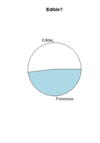
Using the order in this table to create your class category labels, you can build a pie chart.

Pie!

pie(grouped$count,grouped$class, main="Edible?")

And voilà, a pie chart showing the proportions of edible and poisonous mushrooms. It's crucial to get the order of the labels correct, so double-check the label array's order!

Donuts!

A slightly more visually appealing version of a pie chart is a donut chart, which is essentially a pie chart with a hole in the middle. Let's use this method to examine our data.

Take a look at the various habitats where mushrooms grow:

library(dplyr)
habitat=mushrooms %>%
  group_by(habitat) %>%
  summarise(count=n())
View(habitat)

The output is:

habitat	count
Grasses	2148
Leaves	832
Meadows	292
Paths	1144
Urban	368
Waste	192
Wood	3148

Here, the data is grouped by habitat. There are seven habitats listed, so use these as labels for your donut chart:

library(ggplot2)
library(webr)
PieDonut(habitat, aes(habitat, count=count))

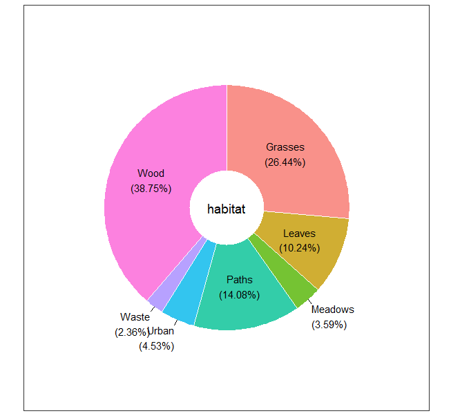
This code uses two libraries: ggplot2 and webr. The PieDonut function from the webr library makes it easy to create a donut chart!

You can also create donut charts in R using only the ggplot2 library. Learn more about it here and give it a try.

Now that you know how to group your data and display it as a pie or donut chart, you can explore other chart types. For example, try a waffle chart, which offers a unique way to visualize quantities.

Waffles!

A waffle chart is a 2D array of squares that visualizes quantities. Let's use it to explore the different mushroom cap colors in this dataset. First, install a helper library called waffle and use it to create your visualization:

install.packages("waffle", repos = "https://cinc.rud.is")

Select a segment of your data to group:

library(dplyr)
cap_color=mushrooms %>%
  group_by(cap.color) %>%
  summarise(count=n())
View(cap_color)

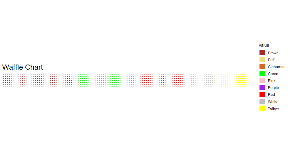
Create a waffle chart by defining labels and grouping your data:

library(waffle)
names(cap_color$count) = paste0(cap_color$cap.color)
waffle((cap_color$count/10), rows = 7, title = "Waffle Chart")+scale_fill_manual(values=c("brown", "#F0DC82", "#D2691E", "green", 
                                                                                     "pink", "purple", "red", "grey", 
                                                                                     "yellow","white"))

The waffle chart clearly shows the proportions of cap colors in the mushroom dataset. Interestingly, there are quite a few green-capped mushrooms!

In this lesson, you learned three ways to visualize proportions. First, group your data into categories, then decide the best way to display it—pie, donut, or waffle. Each method provides a quick and engaging snapshot of the dataset.

🚀 Challenge

Try recreating these fun charts in Charticulator.

Post-lecture quiz

Review & Self Study

It’s not always clear when to use a pie, donut, or waffle chart. Here are some articles to help you decide:

Do some research to learn more about this tricky decision.

Assignment

Try it in Excel

Disclaimer:
This document has been translated using the AI translation service Co-op Translator. While we aim for accuracy, please note that automated translations may include errors or inaccuracies. The original document in its native language should be regarded as the authoritative source. For critical information, professional human translation is advised. We are not responsible for any misunderstandings or misinterpretations resulting from the use of this translation.

10 KiB Raw Permalink Blame History Unescape Escape