
 localizeflow[bot]
081f029c0d
localizeflow[bot]
081f029c0d
|
6 months ago | |
|---|---|---|
| .. | ||
| solution | 9 months ago | |
| working | 9 months ago | |
| README.md | 6 months ago | |
| assignment.md | 6 months ago | |
README.md
Time Series Forecasting wit Support Vector Regressor
For di last lesson, you don learn how to use ARIMA model take make time series predictions. Now, you go dey look Support Vector Regressor model wey be regressor model wey dem dey use predict continuous data.
Pre-lecture quiz
Introduction
For dis lesson, you go sabi one special way to build models wit SVM: Support Vector Machine for regression, or SVR: Support Vector Regressor.
SVR for time series 1
Before you go fit understand why SVR dey important for time series prediction, make we first look some important concepts wey you need sabi:
- Regression: Na supervised learning technique wey dem dey use predict continuous values from di inputs wey dem give. Di idea na to fit curve (or line) for di feature space wey go get di maximum number of data points. Click here to learn more.
- Support Vector Machine (SVM): Na one type of supervised machine learning model wey dem dey use for classification, regression and outliers detection. Di model na hyperplane for di feature space, wey for classification dey act as boundary, and for regression dey act as di best-fit line. For SVM, Kernel function dey usually dey used to transform di dataset to space wey get higher number of dimensions, so dem go dey easy to separate. Click here to learn more about SVMs.
- Support Vector Regressor (SVR): Na one type of SVM wey dey find di best fit line (wey for SVM na hyperplane) wey go get di maximum number of data points.
Why SVR? 1
For di last lesson, you don learn about ARIMA, wey be one statistical linear method wey dey successful for forecasting time series data. But, for many cases, time series data dey get non-linearity, wey linear models no fit map. For dis kind cases, di ability of SVM to handle non-linearity for regression tasks dey make SVR dey successful for time series forecasting.
Exercise - build SVR model
Di first few steps for data preparation na di same as di one for di last lesson on ARIMA.
Open di /working folder for dis lesson and find di notebook.ipynb file.2
-
Run di notebook and import di necessary libraries: 2
import sys
sys.path.append('../../')
import os import warnings import matplotlib.pyplot as plt import numpy as np import pandas as pd import datetime as dt import math from sklearn.svm import SVR from sklearn.preprocessing import MinMaxScaler from common.utils import load_data, mape -
Load di data from di
/data/energy.csvfile into Pandas dataframe and check am: 2energy = load_data('../../data')[['load']] -
Plot all di available energy data from January 2012 to December 2014: 2
energy.plot(y='load', subplots=True, figsize=(15, 8), fontsize=12)
plt.xlabel('timestamp', fontsize=12)
plt.ylabel('load', fontsize=12)
plt.show()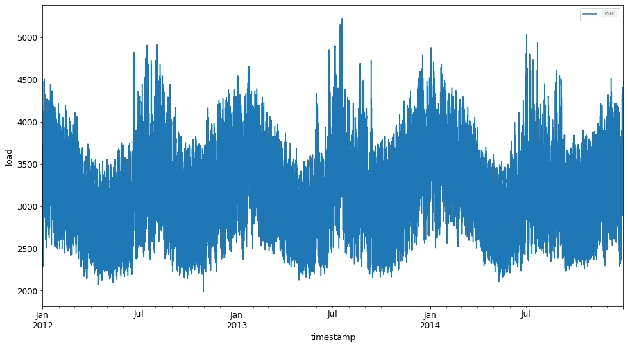
Now, make we build our SVR model.
Create training and testing datasets
Now wey your data don load, you fit separate am into train and test sets. Then you go reshape di data to create time-step based dataset wey SVR go need. You go train your model on di train set. After di model don finish training, you go check di accuracy for di training set, testing set and di full dataset to see di overall performance. You need make sure say di test set dey cover later period for time from di training set to make sure say di model no dey get information from future time periods 2 (dis situation na Overfitting).
-
Allocate two-month period from September 1 to October 31, 2014 to di training set. Di test set go include di two-month period of November 1 to December 31, 2014: 2
train_start_dt = '2014-11-01 00:00:00' test_start_dt = '2014-12-30 00:00:00' -
Visualize di differences: 2
energy[(energy.index < test_start_dt) & (energy.index >= train_start_dt)][['load']].rename(columns={'load':'train'}) \
    .join(energy[test_start_dt:][['load']].rename(columns={'load':'test'}), how='outer') \
    .plot(y=['train', 'test'], figsize=(15, 8), fontsize=12)
plt.xlabel('timestamp', fontsize=12)
plt.ylabel('load', fontsize=12)
plt.show()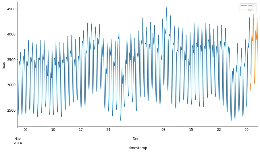
Prepare di data for training
Now, you need prepare di data for training by performing filtering and scaling of your data. Filter your dataset to only include di time periods and columns wey you need, and scale am to make sure say di data dey project for di interval 0,1.
-
Filter di original dataset to include only di time periods wey we mention before per set and only include di needed column 'load' plus di date: 2
train = energy.copy()[(energy.index >= train_start_dt) & (energy.index < test_start_dt)][['load']]
test = energy.copy()[energy.index >= test_start_dt][['load']]

print('Training data shape: ', train.shape)
print('Test data shape: ', test.shape)
Training data shape: (1416, 1) Test data shape: (48, 1) -
Scale di training data to dey range (0, 1): 2
scaler = MinMaxScaler() train['load'] = scaler.fit_transform(train) -
Now, scale di testing data: 2
test['load'] = scaler.transform(test)
Create data wit time-steps 1
For di SVR, you go transform di input data to dey form [batch, timesteps]. So, you go reshape di existing train_data and test_data so dat new dimension go dey wey go refer to di timesteps.
# Converting to numpy arrays
train_data = train.values
test_data = test.values
For dis example, we dey use timesteps = 5. So, di inputs to di model na di data for di first 4 timesteps, and di output go be di data for di 5th timestep.
timesteps=5
Convert training data to 2D tensor using nested list comprehension:
train_data_timesteps=np.array([[j for j in train_data[i:i+timesteps]] for i in range(0,len(train_data)-timesteps+1)])[:,:,0]
train_data_timesteps.shape
(1412, 5)
Convert testing data to 2D tensor:
test_data_timesteps=np.array([[j for j in test_data[i:i+timesteps]] for i in range(0,len(test_data)-timesteps+1)])[:,:,0]
test_data_timesteps.shape
(44, 5)
Select inputs and outputs from training and testing data:
x_train, y_train = train_data_timesteps[:,:timesteps-1],train_data_timesteps[:,[timesteps-1]]
x_test, y_test = test_data_timesteps[:,:timesteps-1],test_data_timesteps[:,[timesteps-1]]

print(x_train.shape, y_train.shape)
print(x_test.shape, y_test.shape)
(1412, 4) (1412, 1)
(44, 4) (44, 1)
Implement SVR 1
Now, na time to implement SVR. To read more about dis implementation, you fit check dis documentation. For our implementation, we go follow dis steps:
- Define di model by calling
SVR()and passing di model hyperparameters: kernel, gamma, c and epsilon - Prepare di model for di training data by calling di
fit()function - Make predictions by calling di
predict()function
Now we go create SVR model. Here we dey use di RBF kernel, and set di hyperparameters gamma, C and epsilon as 0.5, 10 and 0.05 respectively.
model = SVR(kernel='rbf',gamma=0.5, C=10, epsilon = 0.05)
Fit di model on training data 1
model.fit(x_train, y_train[:,0])
SVR(C=10, cache_size=200, coef0=0.0, degree=3, epsilon=0.05, gamma=0.5,
    kernel='rbf', max_iter=-1, shrinking=True, tol=0.001, verbose=False)
Make model predictions 1
y_train_pred = model.predict(x_train).reshape(-1,1)
y_test_pred = model.predict(x_test).reshape(-1,1)

print(y_train_pred.shape, y_test_pred.shape)
(1412, 1) (44, 1)
You don build your SVR! Now we need evaluate am.
Evaluate your model 1
To evaluate, first we go scale back di data to our original scale. Then, to check di performance, we go plot di original and predicted time series plot, and also print di MAPE result.
Scale di predicted and original output:
# Scaling the predictions
y_train_pred = scaler.inverse_transform(y_train_pred)
y_test_pred = scaler.inverse_transform(y_test_pred)

print(len(y_train_pred), len(y_test_pred))
# Scaling the original values
y_train = scaler.inverse_transform(y_train)
y_test = scaler.inverse_transform(y_test)

print(len(y_train), len(y_test))
Check model performance on training and testing data 1
We go extract di timestamps from di dataset to show for di x-axis of our plot. Note say we dey use di first timesteps-1 values as input for di first output, so di timestamps for di output go start after dat.
train_timestamps = energy[(energy.index < test_start_dt) & (energy.index >= train_start_dt)].index[timesteps-1:]
test_timestamps = energy[test_start_dt:].index[timesteps-1:]

print(len(train_timestamps), len(test_timestamps))
1412 44
Plot di predictions for training data:
plt.figure(figsize=(25,6))
plt.plot(train_timestamps, y_train, color = 'red', linewidth=2.0, alpha = 0.6)
plt.plot(train_timestamps, y_train_pred, color = 'blue', linewidth=0.8)
plt.legend(['Actual','Predicted'])
plt.xlabel('Timestamp')
plt.title("Training data prediction")
plt.show()

Print MAPE for training data
print('MAPE for training data: ', mape(y_train_pred, y_train)*100, '%')
MAPE for training data: 1.7195710200875551 %
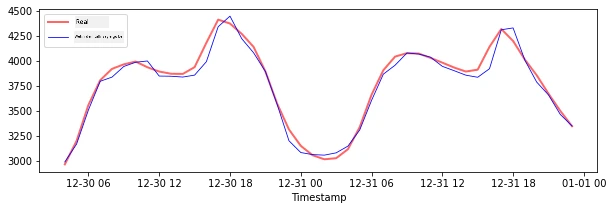
Plot di predictions for testing data
plt.figure(figsize=(10,3))
plt.plot(test_timestamps, y_test, color = 'red', linewidth=2.0, alpha = 0.6)
plt.plot(test_timestamps, y_test_pred, color = 'blue', linewidth=0.8)
plt.legend(['Actual','Predicted'])
plt.xlabel('Timestamp')
plt.show()
Print MAPE for testing data
print('MAPE for testing data: ', mape(y_test_pred, y_test)*100, '%')
MAPE for testing data: 1.2623790187854018 %
🏆 You get very good result for di testing dataset!
Check model performance on full dataset 1
# Extracting load values as numpy array
data = energy.copy().values

# Scaling
data = scaler.transform(data)

# Transforming to 2D tensor as per model input requirement
data_timesteps=np.array([[j for j in data[i:i+timesteps]] for i in range(0,len(data)-timesteps+1)])[:,:,0]
print("Tensor shape: ", data_timesteps.shape)

# Selecting inputs and outputs from data
X, Y = data_timesteps[:,:timesteps-1],data_timesteps[:,[timesteps-1]]
print("X shape: ", X.shape,"\nY shape: ", Y.shape)
Tensor shape:  (26300, 5)
X shape:  (26300, 4)
Y shape:  (26300, 1)
# Make model predictions
Y_pred = model.predict(X).reshape(-1,1)

# Inverse scale and reshape
Y_pred = scaler.inverse_transform(Y_pred)
Y = scaler.inverse_transform(Y)
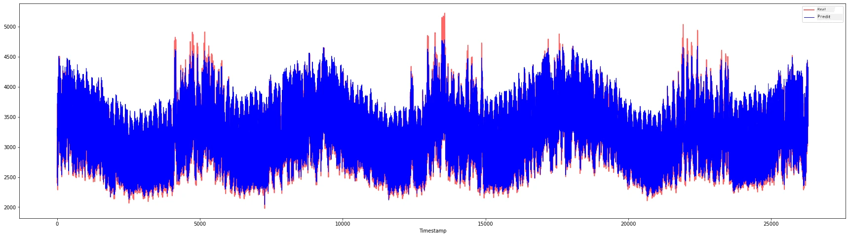
plt.figure(figsize=(30,8))
plt.plot(Y, color = 'red', linewidth=2.0, alpha = 0.6)
plt.plot(Y_pred, color = 'blue', linewidth=0.8)
plt.legend(['Actual','Predicted'])
plt.xlabel('Timestamp')
plt.show()
print('MAPE: ', mape(Y_pred, Y)*100, '%')
MAPE: 2.0572089029888656 %
🏆 Di plots dey nice, e show say di model get good accuracy. Well done!
🚀Challenge
- Try tweak di hyperparameters (gamma, C, epsilon) when you dey create di model and evaluate am on di data to see which set of hyperparameters go give di best results for di testing data. To learn more about dis hyperparameters, you fit check di document here.
- Try use different kernel functions for di model and analyze how dem perform for di dataset. Helpful document dey here.
- Try use different values for
timestepsfor di model to look back to make prediction.
Post-lecture quiz
Review & Self Study
Dis lesson na to introduce di application of SVR for Time Series Forecasting. To read more about SVR, you fit check dis blog. Dis documentation on scikit-learn dey explain more about SVMs in general, SVRs and also other implementation details like di different kernel functions wey fit dey used, and their parameters.
Assignment
Credits
Disclaimer:
Dis dokyument don translate wit AI translation service Co-op Translator. Even though we dey try make am accurate, abeg make you sabi say machine translation fit get mistake or no dey correct well. Di original dokyument for di native language na di main source wey you go trust. For important information, e better make professional human translator check am. We no go fit take blame for any misunderstanding or wrong interpretation wey fit happen because you use dis translation.
-
Di text, code and output for dis section na contribution from @AnirbanMukherjeeXD ↩︎
-
Di text, code and output for dis section na taken from ARIMA ↩︎