
 leestott
0f760e5383
leestott
0f760e5383
|
1 year ago | |
|---|---|---|
| .. | ||
| solution | 1 year ago | |
| working | 1 year ago | |
| README.md | 1 year ago | |
| assignment.md | 1 year ago | |
README.md
使用支持向量回归器进行时间序列预测
在上一节课中,你学习了如何使用 ARIMA 模型进行时间序列预测。现在,你将学习支持向量回归器(SVR)模型,这是一种用于预测连续数据的回归模型。
课前测验
简介
在本节课中,你将了解如何使用SVM:支持向量机进行回归,也就是SVR:支持向量回归器。
时间序列中的 SVR 1
在理解 SVR 在时间序列预测中的重要性之前,你需要了解以下几个重要概念:
- 回归: 一种监督学习技术,用于根据给定的输入集预测连续值。其核心思想是拟合一条曲线(或直线),使其尽可能包含最多的数据点。点击这里了解更多信息。
- 支持向量机(SVM): 一种监督机器学习模型,用于分类、回归和异常值检测。该模型在特征空间中是一条超平面,在分类任务中充当边界,在回归任务中充当最佳拟合线。在 SVM 中,通常使用核函数将数据集转换到更高维度的空间,以便更容易分离。点击这里了解更多关于 SVM 的信息。
- 支持向量回归器(SVR): SVM 的一种类型,用于找到最佳拟合线(在 SVM 中是超平面),使其包含最多的数据点。
为什么选择 SVR? 1
在上一节课中,你学习了 ARIMA,这是一种非常成功的统计线性方法,用于预测时间序列数据。然而,在许多情况下,时间序列数据具有非线性特性,这些特性无法通过线性模型映射。在这种情况下,SVM 在回归任务中考虑数据非线性的能力使得 SVR 在时间序列预测中非常成功。
练习 - 构建 SVR 模型
数据准备的前几步与上一节课关于 ARIMA 的内容相同。
打开本节课中的 /working 文件夹,找到 notebook.ipynb 文件。[ ^2 ]
-
运行 notebook 并导入必要的库:2
import sys
sys.path.append('../../')
import os import warnings import matplotlib.pyplot as plt import numpy as np import pandas as pd import datetime as dt import math from sklearn.svm import SVR from sklearn.preprocessing import MinMaxScaler from common.utils import load_data, mape -
从
/data/energy.csv文件中加载数据到 Pandas 数据框并查看:2energy = load_data('../../data')[['load']] -
绘制 2012 年 1 月至 2014 年 12 月的所有可用能源数据:2
energy.plot(y='load', subplots=True, figsize=(15, 8), fontsize=12)
plt.xlabel('timestamp', fontsize=12)
plt.ylabel('load', fontsize=12)
plt.show()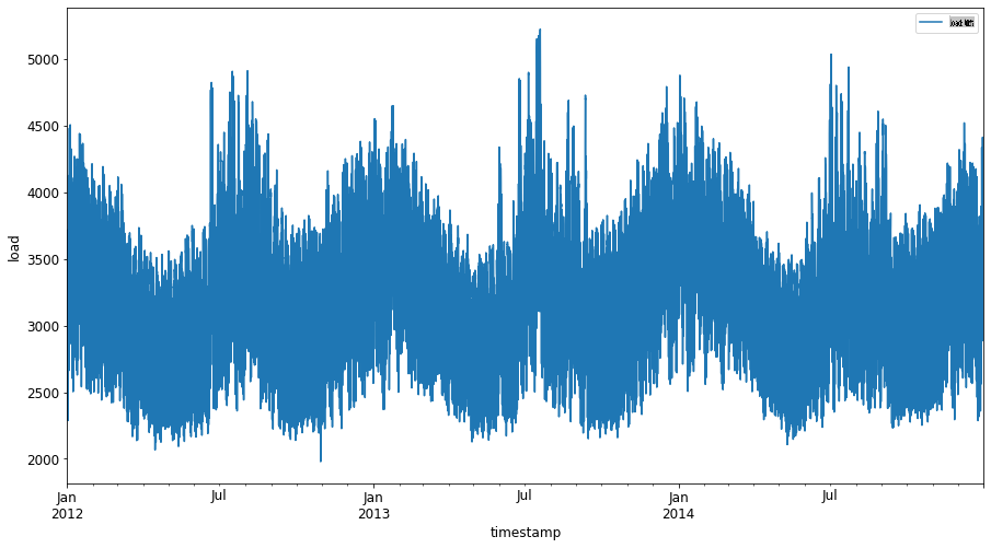
现在,让我们构建 SVR 模型。
创建训练和测试数据集
现在数据已加载,你可以将其分为训练集和测试集。然后,你需要对数据进行重塑,以创建基于时间步长的数据集,这对于 SVR 是必要的。你将在训练集上训练模型。模型训练完成后,你将评估其在训练集、测试集以及完整数据集上的准确性,以查看整体表现。需要确保测试集覆盖的时间段晚于训练集,以确保模型不会从未来时间段中获取信息2(这种情况称为过拟合)。
-
将 2014 年 9 月 1 日至 10 月 31 日的两个月分配给训练集。测试集将包括 2014 年 11 月 1 日至 12 月 31 日的两个月:2
train_start_dt = '2014-11-01 00:00:00' test_start_dt = '2014-12-30 00:00:00' -
可视化差异:2
energy[(energy.index < test_start_dt) & (energy.index >= train_start_dt)][['load']].rename(columns={'load':'train'}) \
    .join(energy[test_start_dt:][['load']].rename(columns={'load':'test'}), how='outer') \
    .plot(y=['train', 'test'], figsize=(15, 8), fontsize=12)
plt.xlabel('timestamp', fontsize=12)
plt.ylabel('load', fontsize=12)
plt.show()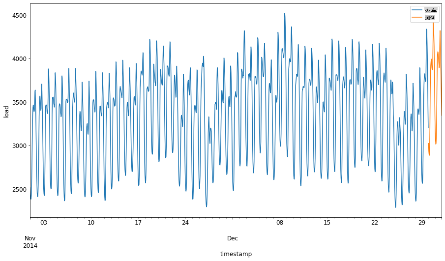
准备训练数据
现在,你需要通过过滤和缩放数据来准备训练数据。过滤数据集以仅包含所需的时间段和列,并进行缩放以确保数据投射到区间 0,1。
-
过滤原始数据集,仅包含上述时间段的每个集合,并仅包含所需的“load”列和日期:2
train = energy.copy()[(energy.index >= train_start_dt) & (energy.index < test_start_dt)][['load']]
test = energy.copy()[energy.index >= test_start_dt][['load']]

print('Training data shape: ', train.shape)
print('Test data shape: ', test.shape)
Training data shape: (1416, 1) Test data shape: (48, 1) -
将训练数据缩放到范围 (0, 1):2
scaler = MinMaxScaler() train['load'] = scaler.fit_transform(train) -
现在,缩放测试数据:2
test['load'] = scaler.transform(test)
创建带时间步长的数据 1
对于 SVR,你需要将输入数据转换为 [batch, timesteps] 的形式。因此,你需要重塑现有的 train_data 和 test_data,以便有一个新的维度表示时间步长。
# Converting to numpy arrays
train_data = train.values
test_data = test.values
在这个例子中,我们取 timesteps = 5。因此,模型的输入是前 4 个时间步长的数据,输出是第 5 个时间步长的数据。
timesteps=5
使用嵌套列表推导将训练数据转换为二维张量:
train_data_timesteps=np.array([[j for j in train_data[i:i+timesteps]] for i in range(0,len(train_data)-timesteps+1)])[:,:,0]
train_data_timesteps.shape
(1412, 5)
将测试数据转换为二维张量:
test_data_timesteps=np.array([[j for j in test_data[i:i+timesteps]] for i in range(0,len(test_data)-timesteps+1)])[:,:,0]
test_data_timesteps.shape
(44, 5)
从训练和测试数据中选择输入和输出:
x_train, y_train = train_data_timesteps[:,:timesteps-1],train_data_timesteps[:,[timesteps-1]]
x_test, y_test = test_data_timesteps[:,:timesteps-1],test_data_timesteps[:,[timesteps-1]]

print(x_train.shape, y_train.shape)
print(x_test.shape, y_test.shape)
(1412, 4) (1412, 1)
(44, 4) (44, 1)
实现 SVR 1
现在是时候实现 SVR 了。要了解更多关于此实现的信息,可以参考此文档。对于我们的实现,我们遵循以下步骤:
- 通过调用
SVR()并传入模型超参数:kernel、gamma、c 和 epsilon 来定义模型 - 通过调用
fit()函数为训练数据准备模型 - 通过调用
predict()函数进行预测
现在我们创建一个 SVR 模型。这里我们使用 RBF 核函数,并将超参数 gamma、C 和 epsilon 分别设置为 0.5、10 和 0.05。
model = SVR(kernel='rbf',gamma=0.5, C=10, epsilon = 0.05)
在训练数据上拟合模型 1
model.fit(x_train, y_train[:,0])
SVR(C=10, cache_size=200, coef0=0.0, degree=3, epsilon=0.05, gamma=0.5,
    kernel='rbf', max_iter=-1, shrinking=True, tol=0.001, verbose=False)
进行模型预测 1
y_train_pred = model.predict(x_train).reshape(-1,1)
y_test_pred = model.predict(x_test).reshape(-1,1)

print(y_train_pred.shape, y_test_pred.shape)
(1412, 1) (44, 1)
你已经构建了 SVR!现在我们需要评估它。
评估你的模型 1
为了评估,首先我们将数据缩放回原始比例。然后,为了检查性能,我们将绘制原始和预测的时间序列图,并打印 MAPE 结果。
将预测和原始输出缩放:
# Scaling the predictions
y_train_pred = scaler.inverse_transform(y_train_pred)
y_test_pred = scaler.inverse_transform(y_test_pred)

print(len(y_train_pred), len(y_test_pred))
# Scaling the original values
y_train = scaler.inverse_transform(y_train)
y_test = scaler.inverse_transform(y_test)

print(len(y_train), len(y_test))
检查模型在训练和测试数据上的表现 1
我们从数据集中提取时间戳,以显示在图表的 x 轴上。注意,我们使用了前 timesteps-1 个值作为第一个输出的输入,因此输出的时间戳将从那之后开始。
train_timestamps = energy[(energy.index < test_start_dt) & (energy.index >= train_start_dt)].index[timesteps-1:]
test_timestamps = energy[test_start_dt:].index[timesteps-1:]

print(len(train_timestamps), len(test_timestamps))
1412 44
绘制训练数据的预测:
plt.figure(figsize=(25,6))
plt.plot(train_timestamps, y_train, color = 'red', linewidth=2.0, alpha = 0.6)
plt.plot(train_timestamps, y_train_pred, color = 'blue', linewidth=0.8)
plt.legend(['Actual','Predicted'])
plt.xlabel('Timestamp')
plt.title("Training data prediction")
plt.show()
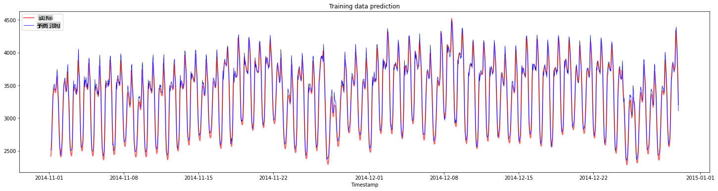
打印训练数据的 MAPE:
print('MAPE for training data: ', mape(y_train_pred, y_train)*100, '%')
MAPE for training data: 1.7195710200875551 %
绘制测试数据的预测:
plt.figure(figsize=(10,3))
plt.plot(test_timestamps, y_test, color = 'red', linewidth=2.0, alpha = 0.6)
plt.plot(test_timestamps, y_test_pred, color = 'blue', linewidth=0.8)
plt.legend(['Actual','Predicted'])
plt.xlabel('Timestamp')
plt.show()
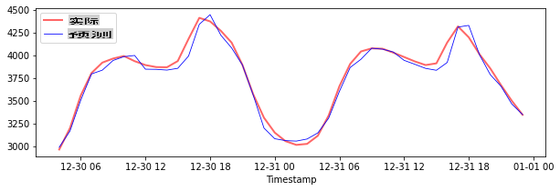
打印测试数据的 MAPE:
print('MAPE for testing data: ', mape(y_test_pred, y_test)*100, '%')
MAPE for testing data: 1.2623790187854018 %
🏆 你在测试数据集上取得了非常好的结果!
检查模型在完整数据集上的表现 1
# Extracting load values as numpy array
data = energy.copy().values

# Scaling
data = scaler.transform(data)

# Transforming to 2D tensor as per model input requirement
data_timesteps=np.array([[j for j in data[i:i+timesteps]] for i in range(0,len(data)-timesteps+1)])[:,:,0]
print("Tensor shape: ", data_timesteps.shape)

# Selecting inputs and outputs from data
X, Y = data_timesteps[:,:timesteps-1],data_timesteps[:,[timesteps-1]]
print("X shape: ", X.shape,"\nY shape: ", Y.shape)
Tensor shape:  (26300, 5)
X shape:  (26300, 4)
Y shape:  (26300, 1)
# Make model predictions
Y_pred = model.predict(X).reshape(-1,1)

# Inverse scale and reshape
Y_pred = scaler.inverse_transform(Y_pred)
Y = scaler.inverse_transform(Y)
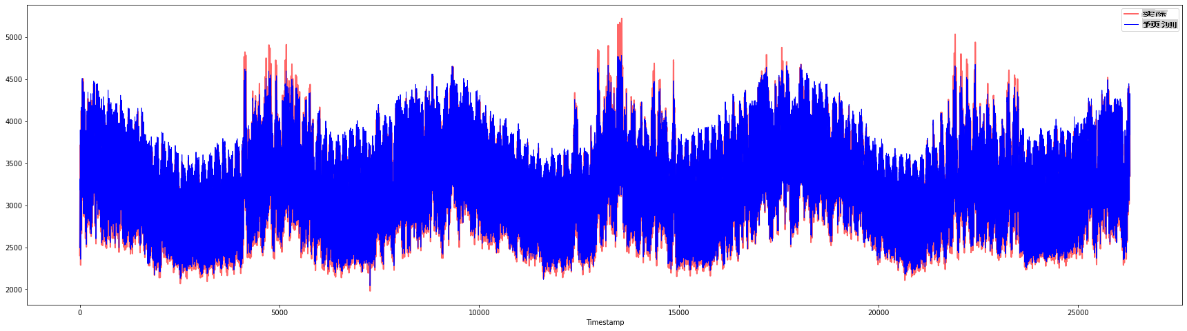
plt.figure(figsize=(30,8))
plt.plot(Y, color = 'red', linewidth=2.0, alpha = 0.6)
plt.plot(Y_pred, color = 'blue', linewidth=0.8)
plt.legend(['Actual','Predicted'])
plt.xlabel('Timestamp')
plt.show()
print('MAPE: ', mape(Y_pred, Y)*100, '%')
MAPE: 2.0572089029888656 %
🏆 非常棒的图表,显示了一个具有良好准确性的模型。干得好!
🚀挑战
- 尝试在创建模型时调整超参数(gamma、C、epsilon),并在数据上进行评估,看看哪组超参数在测试数据上表现最好。要了解更多关于这些超参数的信息,可以参考这里的文档。
- 尝试为模型使用不同的核函数,并分析它们在数据集上的表现。可以参考这里的文档。
- 尝试为模型使用不同的
timesteps值进行回溯预测。
课后测验
复习与自学
本节课旨在介绍 SVR 在时间序列预测中的应用。要了解更多关于 SVR 的信息,可以参考这篇博客。这个scikit-learn 文档提供了关于 SVM 的更全面解释,包括SVR以及其他实现细节,例如可以使用的不同核函数及其参数。
作业
致谢
免责声明:
本文档使用AI翻译服务 Co-op Translator 进行翻译。尽管我们努力确保翻译的准确性,但请注意,自动翻译可能包含错误或不准确之处。原始语言的文档应被视为权威来源。对于重要信息,建议使用专业人工翻译。我们不对因使用此翻译而产生的任何误解或误读承担责任。
-
本节中的文本、代码和输出由 @AnirbanMukherjeeXD 提供 ↩︎