|
|
3 years ago | |
|---|---|---|
| .. | ||
| images | 3 years ago | |
| solution | 3 years ago | |
| translations | 3 years ago | |
| README.md | 3 years ago | |
| assignment.md | 3 years ago | |
| notebook.ipynb | 3 years ago | |
| rlboard.py | 3 years ago | |
README.md
Introduction to Reinforcement Learning and Q-Learning
🎥 Click the image above to hear Dmitry discuss Reinforcement Learning
Pre-lecture quiz
In this lesson, we will explore the world of Peter and the Wolf, inspired by a musical fairy tale by a Russian composer, Sergei Prokofiev. We will use Reinforcement Learning to let Peter explore his environment, collect tasty apples and avoid meeting the wolf.
Prerequisites and Setup
In this lesson, we will be experimenting with some code in Python. So you are expected to be able to run the Jupyter Notebook code from this lesson, either on your computer, or somewhere in the cloud.
You can open the lesson notebook and continue reading the material there, or continue reading here, and run the code in your favorite Python environment.
Note: If you are opening this code from the cloud, you also need to fetch
rlboard.pyfile, because notebook code uses it. Put it into the same directory with the notebook.
Introduction
Reinforcement Learning (RL) is a learning technique that allows us to learn an optimal behavior of an agent in some environment by running many experiments. An agent in this environment should have some goal, defined by a reward function.
The Environment
For simplicity, let's consider Peter's world to be a square board of size width x height, like this:
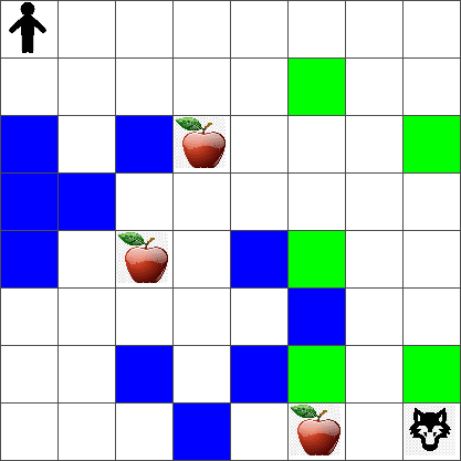
Each cell in this board can either be:
- ground, on which Peter and other creatures can walk
- water, on which you obviously cannot walk
- a tree or grass - a place where you can take some rest
- an apple, which represents something Peter would be glad to find in order to feed himself
- a wolf, which is dangerous and should be avoided
There is a separate Python module, rlboard.py, which contains the code to work with this environment. Because this code is not important for understanding our concepts, we will just import the module and use it to create the sample board (code block 1):
from rlboard import *

width, height = 8,8
m = Board(width,height)
m.randomize(seed=13)
m.plot()
This code should print the picture of the environment similar to the one above.
Actions and Policy
In our example, Peter's goal would be to find an apple, while avoiding the wolf and other obstacles. To do this, he can essentially walk around until he finds and apple. Therefore, at any position he can chose between one of the following actions: up, down, left and right. We will define those actions as a dictionary, and map them to pairs of corresponding coordinate changes. For example, moving right (R) would correspond to a pair (1,0). (code block 2)
actions = { "U" : (0,-1), "D" : (0,1), "L" : (-1,0), "R" : (1,0) }
action_idx = { a : i for i,a in enumerate(actions.keys()) }
The strategy of our agent (Peter) is defined by so-called policy. A policy is a function that returns the action at any given state. In our case, the state of the problem is represented by the board, including the current position of the player.
The goal of reinforcement learning is to eventually learn a good policy that will allow us to solve the problem efficiently. However, as a baseline, let's consider the simplest policy called random walk.
Random walk
Let's first solve our problem by implementing a random walk strategy. With random walk, we will randomly chose the next action from allowed ones, until we reach the apple (code block 3).
def random_policy(m):
    return random.choice(list(actions))

def walk(m,policy,start_position=None):
    n = 0 # number of steps
    # set initial position
    if start_position:
        m.human = start_position
    else:
        m.random_start()
    while True:
        if m.at() == Board.Cell.apple:
            return n # success!
        if m.at() in [Board.Cell.wolf, Board.Cell.water]:
            return -1 # eaten by wolf or drowned
        while True:
            a = actions[policy(m)]
            new_pos = m.move_pos(m.human,a)
            if m.is_valid(new_pos) and m.at(new_pos)!=Board.Cell.water:
                m.move(a) # do the actual move
                break
        n+=1

walk(m,random_policy)
The call to walk should return us the length of corresponding path, which can vary from one run to another. We can run the walk experiment a number of times (say, 100), and print the resulting statistics (code block 4):
def print_statistics(policy):
    s,w,n = 0,0,0
    for _ in range(100):
        z = walk(m,policy)
        if z<0:
            w+=1
        else:
            s += z
            n += 1
    print(f"Average path length = {s/n}, eaten by wolf: {w} times")

print_statistics(random_policy)
Note that the average length of a path is around 30-40 steps, which is quite a lot, given the fact that the average distance to the nearest apple is around 5-6 steps.
You can also see how Peter's movement looks like during random walk:
Reward Function
To make out policy more intelligent, we need to understand which moves are "better" than others. To do this, we need to define our goal. The goal can be defined in terms of reward function, that will return some score value for each state. The higher the number - the better is the reward function. (code block 5)
move_reward = -0.1
goal_reward = 10
end_reward = -10

def reward(m,pos=None):
    pos = pos or m.human
    if not m.is_valid(pos):
        return end_reward
    x = m.at(pos)
    if x==Board.Cell.water or x == Board.Cell.wolf:
        return end_reward
    if x==Board.Cell.apple:
        return goal_reward
    return move_reward
An interesting thing about reward function is that in most of the cases we are only given substantial reward at the end of the game. It means that out algorithm should somehow remember "good" steps that lead to positive reward at the end, and increase their importance. Similarly, all moves that lead to bad results should be discouraged.
Q-Learning
An algorithm that we will discuss here is called Q-Learning. In this algorithm, the policy is defined by a function (or a data structure) called Q-Table. It records the "goodness" of each of the actions in a given state.
It is called Q-Table because it is often convenient to represent it as a table, or multi-dimensional array. Since our board has dimensions width x height, we can represent Q-Table by a numpy array with shape width x height x len(actions): (code block 6)
Q = np.ones((width,height,len(actions)),dtype=np.float)*1.0/len(actions)
Notice that we initially initialize all the values of Q-Table with equal value, in our case - 0.25. That corresponds to the "random walk" policy, because all moves in each state are equally good. We can pass the Q-Table to the plot function in order to visualize the table on the board: m.plot(Q).

In the center of each cell there is an "arrow" that indicates the preferred direction of movement. Since all directions are equal, a dot is displayed.
Now we need to run the simulation, explore our environment, and learn a better distribution of Q-Table values, which will allow us to find the path to the apple much faster.
Essence of Q-Learning: Bellman Equation
Once we start moving, each action will have a corresponding reward, i.e. we can theoretically select the next action based on the highest immediate reward. However, in most of the states the move will not achieve our goal or reaching the apple, and thus we cannot immediately decide which direction is better.
It is not the immediate result that matters, but rather the final result, which we will obtain at the end of the simulation.
In order to account for this delayed reward, we need to use the principles of dynamic programming, which allows us to think about out problem recursively.
Suppose we are now at the state s, and we want to move to the next state s'. By doing so, we will receive the immediate reward r(s,a), defined by reward function, plus some future reward. If we suppose that our Q-Table correctly reflects the "attractiveness" of each action, then at state s' we will chose an action a that corresponds to maximum value of Q(s',a'). Thus, the best possible future reward we could get at state s will be defined as maxa'Q(s',a') (maximum here is computed over all possible actions a' at state s'.
This gives the Bellman formula for calculating the value of Q-Table at state s, given action a:
Here γ is the so-called discount factor that determines to which extent you should prefer current reward over the future reward and vice versa.
Learning Algorithm
Given the equation above, we can now write pseudo-code for our leaning algorithm:
- Initialize Q-Table Q with equal numbers for all states and actions
- Set learning rate α ← 1
- Repeat simulation many times
- Start at random position
- Repeat
- Select an action a at state s
- Execute action by moving to a new state s'
- If we encounter end-of-game condition, or total reward is too small - exit simulation
- Compute reward r at the new state
- Update Q-Function according to Bellman equation: Q(s,a) ← (1-α)Q(s,a)+α(r+γ maxa'Q(s',a'))
- s ← s'
- Update the total reward and decrease α.
Exploit vs. Explore
In the algorithm above, we did not specify how exactly we should choose an action at step 2.1. If we are choosing the action randomly, we will randomly explore the environment, and we are quite likely to die often as well as explore areas where we would not normally go. An alternative approach would be to exploit the Q-Table values that we already know, and thus to choose the best action (with highers Q-Table value) at state s. This, however, will prevent us from exploring other states, and quite likely we might not find the optimal solution.
Thus, the best approach is to balance between exploration and exploitation. This can be done by choosing the action at state s with probabilities proportional to values in Q-Table. In the beginning, when Q-Table values are all the same, it would correspond to a random selection, but as we learn more about our environment, we would be more likely to follow the optimal route while allowing the agent to choose the unexplored path once in a while.
Python Implementation
Now we are ready to implement the learning algorithm. Before that, we also need some function that will convert arbitrary numbers in the Q-Table into a vector of probabilities for corresponding actions: (code block 7)
def probs(v,eps=1e-4):
    v = v-v.min()+eps
    v = v/v.sum()
    return v
We add a few eps to the original vector in order to avoid division by 0 in the initial case, when all components of the vector are identical.
The actual learning algorithm we will run for 5000 experiments, also called epochs: (code block 8)
for epoch in range(5000):

    # Pick initial point
    m.random_start()

    # Start travelling
    n=0
    cum_reward = 0
    while True:
        x,y = m.human
        v = probs(Q[x,y])
        a = random.choices(list(actions),weights=v)[0]
        dpos = actions[a]
        m.move(dpos)
        r = reward(m)
        cum_reward += r
        if r==end_reward or cum_reward < -1000:
            lpath.append(n)
            break
        alpha = np.exp(-n / 10e5)
        gamma = 0.5
        ai = action_idx[a]
        Q[x,y,ai] = (1 - alpha) * Q[x,y,ai] + alpha * (r + gamma * Q[x+dpos[0], y+dpos[1]].max())
        n+=1
After executing this algorithm, Q-Table should be updated with values that define the attractiveness of different actions at each step. We can try to visualize Q-Table by plotting a vector at each cell that will point in the desired direction of movement. For simplicity, we draw a small circle instead of an arrow head.

Checking the Policy
Since Q-Table lists the "attractiveness" of each action at each state, it is quite easy to use it to define the efficient navigation in our world. In the simplest case, we can select the action corresponding to the highest Q-Table value: (code block 9)
def qpolicy_strict(m):
        x,y = m.human
        v = probs(Q[x,y])
        a = list(actions)[np.argmax(v)]
        return a

walk(m,qpolicy_strict)
If you try the code above several times, you may notice that sometimes it "hangs", and you need to press the STOP button in the notebook to interrupt it. This happens because there could be situations when two states "point" to each other in terms of optimal Q-Value, in which case the agents ends up moving between those states indefinitely.
🚀Challenge
Task 1: Modify the
walkfunction to limit the maximum length of path by a certain number of steps (say, 100), and watch the code above return this value from time to time.
Task 2: Modify the
walkfunction so that it does not go back to the places where is has already been previously. This will preventwalkfrom looping, however, the agent can still end up being "trapped" in a location from which it is unable to escape.
Navigation
Better navigation policy would be the one that we have used during training, which combines exploitation and exploration. In this policy, we will select each action with a certain probability, proportional to the values in Q-Table. This strategy may still result in the agent returning back to the position it has already explored, but, as you can see from the code below, it results in very short average path to the desired location (remember that print_statistics runs the simulation 100 times): (code block 10)
def qpolicy(m):
        x,y = m.human
        v = probs(Q[x,y])
        a = random.choices(list(actions),weights=v)[0]
        return a

print_statistics(qpolicy)
After running this code, you should get a much smaller average path length than before, in the range of 3-6.
Investigating the learning process
As we have mentioned, the learning process is a balance between exploration and exploration of gained knowledge about the structure of problem space. We have seen that the result of learning (the ability to help an agent to find a short path to the goal) has improved, but it is also interesting to observe how the average path length behaves during the learning process:

What we see here is that at first the average path length increases. This is probably due to the fact that when we know nothing about the environment we are likely to get trapped into bad states, water or wolf. As we learn more and start using this knowledge, we can explore the environment for longer, but we still do not know where the apples are very well.
Once we learn enough, it becomes easier for the agent to achieve the goal, and the path length starts to decrease. However, we are still open to exploration, so we often diverge away from the best path, and explore new options, making the path longer than optimal.
What we also observe on this graph, is that at some point the length increased abruptly. This indicates stochastic nature of the process, and that we can at some point "spoil" the Q-Table coefficients by overwriting them with new values. This ideally should be minimized by decreasing learning rate (i.e. towards the end of training we only adjust Q-Table values by a small value).
Overall, it is important to remember that the success and quality of the learning process significantly depends on parameters, such as leaning rate, learning rate decay and discount factor. Those are often called hyperparameters, to distinguish them from parameters which we optimize during training (eg. Q-Table coefficients). The process of finding best hyperparameter values is called hyperparameter optimization, and it deserves a separate topic.