|
|
2 weeks ago | |
|---|---|---|
| .. | ||
| solution | 3 weeks ago | |
| working | 3 weeks ago | |
| README.md | 2 weeks ago | |
| assignment.md | 3 weeks ago | |
README.md
サポートベクター回帰による時系列予測
前回のレッスンでは、ARIMAモデルを使用して時系列予測を行う方法を学びました。今回は、連続データを予測するために使用される回帰モデルであるサポートベクター回帰(Support Vector Regressor)モデルについて学びます。
事前クイズ
はじめに
このレッスンでは、回帰のためのSVM: Support Vector Machineを使用してモデルを構築する具体的な方法を学びます。これをSVR: Support Vector Regressorと呼びます。
時系列におけるSVR 1
時系列予測におけるSVRの重要性を理解する前に、以下の重要な概念を知っておく必要があります:
- 回帰: 与えられた入力セットから連続値を予測する教師あり学習技術。特徴空間内で最大数のデータポイントを持つ曲線(または直線)をフィットさせることが目的です。詳細はこちら。
- サポートベクターマシン (SVM): 分類、回帰、外れ値検出に使用される教師あり機械学習モデルの一種。モデルは特徴空間内のハイパープレーンであり、分類の場合は境界として機能し、回帰の場合は最適なフィットラインとして機能します。SVMでは、カーネル関数を使用してデータセットをより高次元の空間に変換し、分離しやすくします。詳細はこちら。
- サポートベクター回帰 (SVR): SVMの一種で、最大数のデータポイントを持つ最適なフィットライン(SVMの場合はハイパープレーン)を見つけることを目的としています。
なぜSVRなのか? 1
前回のレッスンでは、時系列データを予測するための非常に成功した統計的線形手法であるARIMAについて学びました。しかし、多くの場合、時系列データには非線形性が含まれており、線形モデルでは対応できません。そのような場合、回帰タスクにおいてデータの非線形性を考慮するSVMの能力が、時系列予測においてSVRを成功させる要因となります。
演習 - SVRモデルを構築する
データ準備の最初のステップは、前回のARIMAレッスンと同じです。
このレッスンの/workingフォルダーを開き、notebook.ipynbファイルを見つけてください。2
-
ノートブックを実行し、必要なライブラリをインポートします: 2
import sys
sys.path.append('../../')
import os import warnings import matplotlib.pyplot as plt import numpy as np import pandas as pd import datetime as dt import math from sklearn.svm import SVR from sklearn.preprocessing import MinMaxScaler from common.utils import load_data, mape -
/data/energy.csvファイルからデータをPandasデータフレームに読み込み、確認します: 2energy = load_data('../../data')[['load']] -
2012年1月から2014年12月までの利用可能なエネルギーデータをプロットします: 2
energy.plot(y='load', subplots=True, figsize=(15, 8), fontsize=12)
plt.xlabel('timestamp', fontsize=12)
plt.ylabel('load', fontsize=12)
plt.show()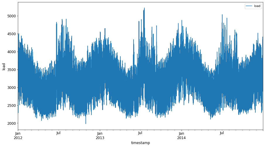
では、SVRモデルを構築しましょう。
トレーニングとテストデータセットを作成する
データが読み込まれたので、トレーニングセットとテストセットに分割します。その後、SVRに必要なタイムステップベースのデータセットを作成するためにデータを再構成します。トレーニングセットでモデルをトレーニングします。トレーニングが完了したら、トレーニングセット、テストセット、そして全データセットでモデルの精度を評価し、全体的なパフォーマンスを確認します。テストセットがトレーニングセットより後の期間をカバーするようにして、モデルが将来の期間から情報を取得しないようにする必要があります2(これを過学習と呼びます)。
-
2014年9月1日から10月31日までの2か月間をトレーニングセットに割り当てます。テストセットには2014年11月1日から12月31日までの2か月間を含めます: 2
train_start_dt = '2014-11-01 00:00:00' test_start_dt = '2014-12-30 00:00:00' -
違いを可視化します: 2
energy[(energy.index < test_start_dt) & (energy.index >= train_start_dt)][['load']].rename(columns={'load':'train'}) \
    .join(energy[test_start_dt:][['load']].rename(columns={'load':'test'}), how='outer') \
    .plot(y=['train', 'test'], figsize=(15, 8), fontsize=12)
plt.xlabel('timestamp', fontsize=12)
plt.ylabel('load', fontsize=12)
plt.show()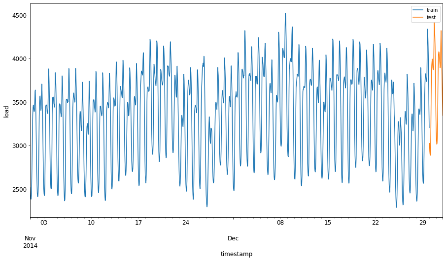
トレーニングのためのデータ準備
次に、データをフィルタリングしてスケーリングすることでトレーニングの準備をします。必要な期間と列のみを含むようにデータセットをフィルタリングし、データを0から1の範囲に投影するようにスケーリングします。
-
元のデータセットをフィルタリングして、前述の期間ごとのセットと必要な列「load」と日付のみを含むようにします: 2
train = energy.copy()[(energy.index >= train_start_dt) & (energy.index < test_start_dt)][['load']]
test = energy.copy()[energy.index >= test_start_dt][['load']]

print('Training data shape: ', train.shape)
print('Test data shape: ', test.shape)
Training data shape: (1416, 1) Test data shape: (48, 1) -
トレーニングデータを(0, 1)の範囲にスケーリングします: 2
scaler = MinMaxScaler() train['load'] = scaler.fit_transform(train) -
次に、テストデータをスケーリングします: 2
test['load'] = scaler.transform(test)
タイムステップを使用したデータ作成 1
SVRでは、入力データを[batch, timesteps]の形式に変換します。そのため、既存のtrain_dataとtest_dataを再構成し、新しい次元(タイムステップ)を追加します。
# Converting to numpy arrays
train_data = train.values
test_data = test.values
この例では、timesteps = 5を使用します。つまり、モデルへの入力は最初の4つのタイムステップのデータであり、出力は5番目のタイムステップのデータになります。
timesteps=5
ネストされたリスト内包表記を使用してトレーニングデータを2Dテンソルに変換します:
train_data_timesteps=np.array([[j for j in train_data[i:i+timesteps]] for i in range(0,len(train_data)-timesteps+1)])[:,:,0]
train_data_timesteps.shape
(1412, 5)
テストデータを2Dテンソルに変換します:
test_data_timesteps=np.array([[j for j in test_data[i:i+timesteps]] for i in range(0,len(test_data)-timesteps+1)])[:,:,0]
test_data_timesteps.shape
(44, 5)
トレーニングデータとテストデータから入力と出力を選択します:
x_train, y_train = train_data_timesteps[:,:timesteps-1],train_data_timesteps[:,[timesteps-1]]
x_test, y_test = test_data_timesteps[:,:timesteps-1],test_data_timesteps[:,[timesteps-1]]

print(x_train.shape, y_train.shape)
print(x_test.shape, y_test.shape)
(1412, 4) (1412, 1)
(44, 4) (44, 1)
SVRの実装 1
次に、SVRを実装します。この実装について詳しく知りたい場合は、こちらのドキュメントを参照してください。今回の実装では以下の手順を行います:
SVR()を呼び出し、カーネル、ガンマ、C、イプシロンなどのモデルハイパーパラメータを渡してモデルを定義します。fit()関数を呼び出してトレーニングデータにモデルを適用します。predict()関数を呼び出して予測を行います。
ここではRBFカーネルを使用し、ハイパーパラメータのガンマ、C、イプシロンをそれぞれ0.5、10、0.05に設定します。
model = SVR(kernel='rbf',gamma=0.5, C=10, epsilon = 0.05)
トレーニングデータにモデルを適用 1
model.fit(x_train, y_train[:,0])
SVR(C=10, cache_size=200, coef0=0.0, degree=3, epsilon=0.05, gamma=0.5,
    kernel='rbf', max_iter=-1, shrinking=True, tol=0.001, verbose=False)
モデル予測を行う 1
y_train_pred = model.predict(x_train).reshape(-1,1)
y_test_pred = model.predict(x_test).reshape(-1,1)

print(y_train_pred.shape, y_test_pred.shape)
(1412, 1) (44, 1)
SVRを構築しました!次に評価を行います。
モデルを評価する 1
評価では、まずデータを元のスケールに戻します。その後、性能を確認するために、元の時系列データと予測データのプロットを作成し、MAPE結果を出力します。
予測値と元の出力をスケールバックします:
# Scaling the predictions
y_train_pred = scaler.inverse_transform(y_train_pred)
y_test_pred = scaler.inverse_transform(y_test_pred)

print(len(y_train_pred), len(y_test_pred))
# Scaling the original values
y_train = scaler.inverse_transform(y_train)
y_test = scaler.inverse_transform(y_test)

print(len(y_train), len(y_test))
トレーニングデータとテストデータでモデル性能を確認 1
データセットからタイムスタンプを抽出し、プロットのx軸に表示します。最初のtimesteps-1値を最初の出力の入力として使用しているため、出力のタイムスタンプはその後から始まります。
train_timestamps = energy[(energy.index < test_start_dt) & (energy.index >= train_start_dt)].index[timesteps-1:]
test_timestamps = energy[test_start_dt:].index[timesteps-1:]

print(len(train_timestamps), len(test_timestamps))
1412 44
トレーニングデータの予測をプロットします:
plt.figure(figsize=(25,6))
plt.plot(train_timestamps, y_train, color = 'red', linewidth=2.0, alpha = 0.6)
plt.plot(train_timestamps, y_train_pred, color = 'blue', linewidth=0.8)
plt.legend(['Actual','Predicted'])
plt.xlabel('Timestamp')
plt.title("Training data prediction")
plt.show()
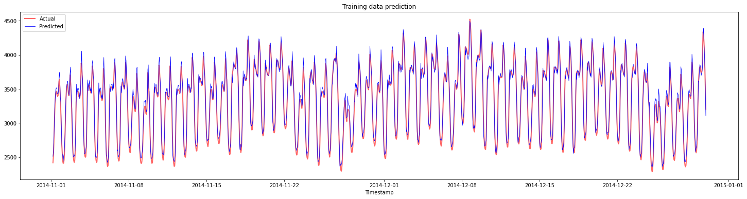
トレーニングデータのMAPEを出力します:
print('MAPE for training data: ', mape(y_train_pred, y_train)*100, '%')
MAPE for training data: 1.7195710200875551 %
テストデータの予測をプロットします:
plt.figure(figsize=(10,3))
plt.plot(test_timestamps, y_test, color = 'red', linewidth=2.0, alpha = 0.6)
plt.plot(test_timestamps, y_test_pred, color = 'blue', linewidth=0.8)
plt.legend(['Actual','Predicted'])
plt.xlabel('Timestamp')
plt.show()
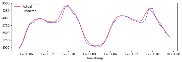
テストデータのMAPEを出力します:
print('MAPE for testing data: ', mape(y_test_pred, y_test)*100, '%')
MAPE for testing data: 1.2623790187854018 %
🏆 テストデータセットで非常に良い結果が得られました!
全データセットでモデル性能を確認 1
# Extracting load values as numpy array
data = energy.copy().values

# Scaling
data = scaler.transform(data)

# Transforming to 2D tensor as per model input requirement
data_timesteps=np.array([[j for j in data[i:i+timesteps]] for i in range(0,len(data)-timesteps+1)])[:,:,0]
print("Tensor shape: ", data_timesteps.shape)

# Selecting inputs and outputs from data
X, Y = data_timesteps[:,:timesteps-1],data_timesteps[:,[timesteps-1]]
print("X shape: ", X.shape,"\nY shape: ", Y.shape)
Tensor shape:  (26300, 5)
X shape:  (26300, 4)
Y shape:  (26300, 1)
# Make model predictions
Y_pred = model.predict(X).reshape(-1,1)

# Inverse scale and reshape
Y_pred = scaler.inverse_transform(Y_pred)
Y = scaler.inverse_transform(Y)
plt.figure(figsize=(30,8))
plt.plot(Y, color = 'red', linewidth=2.0, alpha = 0.6)
plt.plot(Y_pred, color = 'blue', linewidth=0.8)
plt.legend(['Actual','Predicted'])
plt.xlabel('Timestamp')
plt.show()
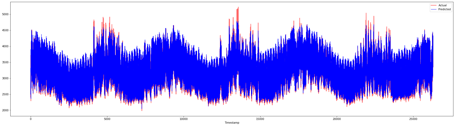
print('MAPE: ', mape(Y_pred, Y)*100, '%')
MAPE: 2.0572089029888656 %
🏆 素晴らしいプロットで、精度の高いモデルを示しています。よくできました!
🚀チャレンジ
- モデルを作成する際にハイパーパラメータ(ガンマ、C、イプシロン)を調整し、テストデータで評価して、どのハイパーパラメータセットが最良の結果をもたらすか確認してください。これらのハイパーパラメータについて詳しく知りたい場合は、こちらのドキュメントを参照してください。
- モデルに異なるカーネル関数を使用し、それらの性能をデータセットで分析してください。役立つドキュメントはこちらにあります。
- モデルが予測を行う際に参照する
timestepsの値を変更してみてください。
事後クイズ
復習と自己学習
このレッスンでは、時系列予測におけるSVRの応用を紹介しました。SVRについてさらに詳しく知りたい場合は、このブログを参照してください。このscikit-learnのドキュメントでは、一般的なSVM、SVR、および使用可能な異なるカーネル関数やそのパラメータなどの実装詳細について包括的な説明が提供されています。
課題
クレジット
免責事項:
この文書は、AI翻訳サービス Co-op Translator を使用して翻訳されています。正確性を期すよう努めておりますが、自動翻訳には誤りや不正確な表現が含まれる可能性があります。元の言語で記載された原文を公式な情報源としてご参照ください。重要な情報については、専門の人間による翻訳を推奨します。本翻訳の利用に起因する誤解や誤認について、当社は一切の責任を負いません。
-
このセクションのテキスト、コード、および出力は@AnirbanMukherjeeXDによって寄稿されました。 ↩︎