|
|
3 weeks ago | |
|---|---|---|
| .. | ||
| solution | 3 weeks ago | |
| README.md | 3 weeks ago | |
| assignment.md | 3 weeks ago | |
| notebook.ipynb | 3 weeks ago | |
README.md
Prerequisites
In this lesson, we will use a library called OpenAI Gym to simulate different environments. You can run the code for this lesson locally (e.g., using Visual Studio Code), in which case the simulation will open in a new window. If you're running the code online, you may need to make some adjustments, as described here.
OpenAI Gym
In the previous lesson, the rules of the game and the state were defined by the Board class that we created ourselves. Here, we will use a specialized simulation environment to simulate the physics of the balancing pole. One of the most popular simulation environments for training reinforcement learning algorithms is called Gym, maintained by OpenAI. Using Gym, we can create various environments, ranging from cartpole simulations to Atari games.
Note: You can explore other environments available in OpenAI Gym here.
First, let's install Gym and import the required libraries (code block 1):
import sys
!{sys.executable} -m pip install gym

import gym
import matplotlib.pyplot as plt
import numpy as np
import random
Exercise - Initialize a CartPole Environment
To work on the cartpole balancing problem, we need to initialize the corresponding environment. Each environment is associated with:
-
Observation space, which defines the structure of the information we receive from the environment. For the cartpole problem, we receive the position of the pole, velocity, and other values.
-
Action space, which defines the possible actions. In this case, the action space is discrete and consists of two actions: left and right. (code block 2)
-
To initialize the environment, type the following code:
env = gym.make("CartPole-v1")
print(env.action_space)
print(env.observation_space)
print(env.action_space.sample())
To understand how the environment works, let's run a short simulation for 100 steps. At each step, we provide an action to be taken—here, we randomly select an action from action_space.
-
Run the code below and observe the results.
✅ It's recommended to run this code on a local Python installation! (code block 3)
env.reset()

for i in range(100):
   env.render()
   env.step(env.action_space.sample())
env.close()
You should see something similar to this image:

-
During the simulation, we need to gather observations to decide on the next action. The
stepfunction returns the current observations, a reward value, and a flag (done) indicating whether the simulation should continue or stop: (code block 4)env.reset() done = False while not done: env.render() obs, rew, done, info = env.step(env.action_space.sample()) print(f"{obs} -> {rew}") env.close()You will see output similar to this in the notebook:
[ 0.03403272 -0.24301182  0.02669811  0.2895829 ] -> 1.0
[ 0.02917248 -0.04828055  0.03248977  0.00543839] -> 1.0
[ 0.02820687  0.14636075  0.03259854 -0.27681916] -> 1.0
[ 0.03113408  0.34100283  0.02706215 -0.55904489] -> 1.0
[ 0.03795414  0.53573468  0.01588125 -0.84308041] -> 1.0
...
[ 0.17299878  0.15868546 -0.20754175 -0.55975453] -> 1.0
[ 0.17617249  0.35602306 -0.21873684 -0.90998894] -> 1.0
The observation vector returned at each step contains the following values:
- Position of the cart
- Velocity of the cart
- Angle of the pole
- Rotation rate of the pole
-
Retrieve the minimum and maximum values of these numbers: (code block 5)
print(env.observation_space.low)
print(env.observation_space.high)
You may also notice that the reward value at each simulation step is always 1. This is because the goal is to survive as long as possible, i.e., to keep the pole reasonably vertical for the longest time.
✅ The CartPole simulation is considered solved if we achieve an average reward of 195 over 100 consecutive trials.
State Discretization
In Q-Learning, we need to build a Q-Table that defines the actions for each state. To do this, the state must be discrete, meaning it should consist of a finite number of discrete values. Therefore, we need to discretize our observations, mapping them to a finite set of states.
There are a few ways to achieve this:
- Divide into bins: If we know the range of a value, we can divide it into a number of bins and replace the value with the bin number it belongs to. This can be done using the numpy
digitizemethod. This approach gives precise control over the state size, as it depends on the number of bins chosen for discretization.
✅ Alternatively, we can use linear interpolation to map values to a finite interval (e.g., from -20 to 20) and then convert them to integers by rounding. This approach offers less control over the state size, especially if the exact ranges of input values are unknown. For example, in our case, 2 out of 4 values lack upper/lower bounds, which could result in an infinite number of states.
In this example, we'll use the second approach. As you'll notice later, despite undefined upper/lower bounds, these values rarely exceed certain finite intervals, making states with extreme values very rare.
-
Here's a function that takes the observation from our model and produces a tuple of 4 integer values: (code block 6)
def discretize(x): return tuple((x/np.array([0.25, 0.25, 0.01, 0.1])).astype(np.int)) -
Let's also explore another discretization method using bins: (code block 7)
def create_bins(i,num): return np.arange(num+1)*(i[1]-i[0])/num+i[0] print("Sample bins for interval (-5,5) with 10 bins\n",create_bins((-5,5),10)) ints = [(-5,5),(-2,2),(-0.5,0.5),(-2,2)] # intervals of values for each parameter nbins = [20,20,10,10] # number of bins for each parameter bins = [create_bins(ints[i],nbins[i]) for i in range(4)] def discretize_bins(x): return tuple(np.digitize(x[i],bins[i]) for i in range(4)) -
Now, run a short simulation and observe the discrete environment values. Feel free to try both
discretizeanddiscretize_binsto see if there's a difference.✅
discretize_binsreturns the bin number, which is 0-based. For input values around 0, it returns the middle bin number (10). Indiscretize, we didn't constrain the output range, allowing negative values, so 0 corresponds directly to 0. (code block 8)env.reset() done = False while not done: #env.render() obs, rew, done, info = env.step(env.action_space.sample()) #print(discretize_bins(obs)) print(discretize(obs)) env.close()✅ Uncomment the line starting with
env.renderif you want to visualize the environment's execution. Otherwise, you can run it in the background for faster execution. We'll use this "invisible" execution during the Q-Learning process.
The Q-Table Structure
In the previous lesson, the state was a simple pair of numbers ranging from 0 to 8, making it convenient to represent the Q-Table as a numpy tensor with a shape of 8x8x2. If we use bin discretization, the size of our state vector is also known, so we can use a similar approach and represent the state as an array with a shape of 20x20x10x10x2 (where 2 corresponds to the action space dimension, and the first dimensions represent the number of bins chosen for each parameter in the observation space).
However, sometimes the precise dimensions of the observation space are unknown. In the case of the discretize function, we can't guarantee that the state will remain within certain limits, as some original values are unbounded. Therefore, we'll use a slightly different approach and represent the Q-Table as a dictionary.
-
Use the pair (state, action) as the dictionary key, with the corresponding Q-Table entry value as the value. (code block 9)
Q = {}
actions = (0,1)

def qvalues(state):
    return [Q.get((state,a),0) for a in actions]
Here, we also define a function
qvalues()that returns a list of Q-Table values for a given state corresponding to all possible actions. If the entry isn't present in the Q-Table, it defaults to 0.
Let's Start Q-Learning
Now it's time to teach Peter how to balance!
-
First, set some hyperparameters: (code block 10)
# hyperparameters
alpha = 0.3
gamma = 0.9
epsilon = 0.90
Here:
alphais the learning rate, which determines how much we adjust the current Q-Table values at each step. In the previous lesson, we started with 1 and gradually decreasedalphaduring training. In this example, we'll keep it constant for simplicity, but you can experiment with adjustingalphalater.gammais the discount factor, which indicates how much we prioritize future rewards over immediate rewards.epsilonis the exploration/exploitation factor, which decides whether to favor exploration or exploitation. In our algorithm, we'll select the next action based on Q-Table values inepsilonpercent of cases, and choose a random action in the remaining cases. This helps explore areas of the search space that haven't been visited yet.
✅ In terms of balancing, choosing a random action (exploration) acts like a random push in the wrong direction, forcing the pole to learn how to recover balance from these "mistakes."
Improve the Algorithm
We can make two improvements to the algorithm from the previous lesson:
-
Calculate average cumulative reward over multiple simulations. We'll print progress every 5000 iterations and average the cumulative reward over that period. If we achieve more than 195 points, we can consider the problem solved, exceeding the required quality.
-
Track maximum average cumulative reward,
Qmax, and store the Q-Table corresponding to that result. During training, you'll notice that the average cumulative reward sometimes drops, so we want to preserve the Q-Table values corresponding to the best model observed.
-
Collect all cumulative rewards from each simulation in the
rewardsvector for later plotting. (code block 11)def probs(v,eps=1e-4): v = v-v.min()+eps v = v/v.sum() return v Qmax = 0 cum_rewards = [] rewards = [] for epoch in range(100000): obs = env.reset() done = False cum_reward=0 # == do the simulation == while not done: s = discretize(obs) if random.random()<epsilon: # exploitation - chose the action according to Q-Table probabilities v = probs(np.array(qvalues(s))) a = random.choices(actions,weights=v)[0] else: # exploration - randomly chose the action a = np.random.randint(env.action_space.n) obs, rew, done, info = env.step(a) cum_reward+=rew ns = discretize(obs) Q[(s,a)] = (1 - alpha) * Q.get((s,a),0) + alpha * (rew + gamma * max(qvalues(ns))) cum_rewards.append(cum_reward) rewards.append(cum_reward) # == Periodically print results and calculate average reward == if epoch%5000==0: print(f"{epoch}: {np.average(cum_rewards)}, alpha={alpha}, epsilon={epsilon}") if np.average(cum_rewards) > Qmax: Qmax = np.average(cum_rewards) Qbest = Q cum_rewards=[]
What you'll notice from the results:
-
Close to the goal: We're very close to achieving the goal of 195 cumulative rewards over 100+ consecutive runs, or we may have already achieved it! Even if the numbers are slightly lower, we can't be certain because we're averaging over 5000 runs, while the formal criteria require only 100 runs.
-
Reward drops: Sometimes the reward starts to drop, indicating that we might overwrite well-learned Q-Table values with worse ones.
This observation becomes clearer when we plot the training progress.
Plotting Training Progress
During training, we collected cumulative reward values at each iteration in the rewards vector. Here's how it looks when plotted against the iteration number:
plt.plot(rewards)
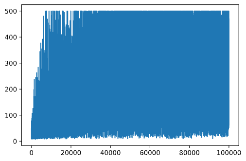
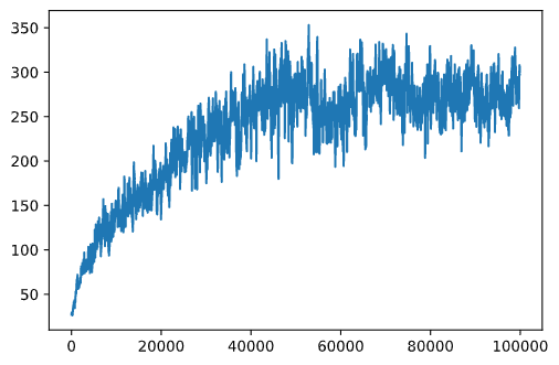
This graph doesn't provide much insight due to the stochastic nature of the training process, which causes session lengths to vary significantly. To make the graph more meaningful, we can calculate the running average over a series of experiments, say 100. This can be done conveniently using np.convolve: (code block 12)
def running_average(x,window):
    return np.convolve(x,np.ones(window)/window,mode='valid')

plt.plot(running_average(rewards,100))
Adjusting Hyperparameters
To make learning more stable, we can adjust some hyperparameters during training. Specifically:
-
Learning rate (
alpha): Start with values close to 1 and gradually decrease it. Over time, as the Q-Table values become more reliable, adjustments should be smaller to avoid overwriting good values completely. -
Exploration factor (
epsilon): Gradually increaseepsilonto explore less and exploit more. It might be better to start with a lowerepsilonvalue and increase it to nearly 1 over time.
Task 1: Experiment with the hyperparameter values and see if you can achieve a higher cumulative reward. Are you reaching above 195? Task 2: To formally solve the problem, you need to achieve an average reward of 195 across 100 consecutive runs. Track this during training to ensure the problem is officially solved!
Seeing the result in action
It’s fascinating to observe how the trained model performs. Let’s run the simulation and use the same action selection strategy as during training, sampling based on the probability distribution in the Q-Table: (code block 13)
obs = env.reset()
done = False
while not done:
   s = discretize(obs)
   env.render()
   v = probs(np.array(qvalues(s)))
   a = random.choices(actions,weights=v)[0]
   obs,_,done,_ = env.step(a)
env.close()
You should see something similar to this:
🚀Challenge
Task 3: In this example, we used the final version of the Q-Table, which might not be the optimal one. Remember, we saved the best-performing Q-Table in the
Qbestvariable! Try running the same example using the best-performing Q-Table by copyingQbestintoQand observe if there’s any noticeable difference.
Task 4: In this example, we didn’t always select the best action at each step but instead sampled actions based on the corresponding probability distribution. Would it be better to always choose the best action—the one with the highest Q-Table value? This can be achieved using the
np.argmaxfunction to identify the action number with the highest Q-Table value. Implement this strategy and check if it improves the balancing performance.
Post-lecture quiz
Assignment
Conclusion
We’ve now learned how to train agents to achieve strong results simply by providing them with a reward function that defines the desired state of the game and allowing them to intelligently explore the search space. We successfully applied the Q-Learning algorithm in both discrete and continuous environments, though with discrete actions.
It’s also crucial to study scenarios where the action space is continuous and the observation space is more complex, such as an image from an Atari game screen. In such cases, more advanced machine learning techniques, like neural networks, are often required to achieve good results. These advanced topics will be covered in our upcoming, more advanced AI course.
Disclaimer:
This document has been translated using the AI translation service Co-op Translator. While we strive for accuracy, please note that automated translations may contain errors or inaccuracies. The original document in its native language should be regarded as the authoritative source. For critical information, professional human translation is recommended. We are not responsible for any misunderstandings or misinterpretations resulting from the use of this translation.