History

leestott fad44a68c4 🌐 Update translations via Co-op Translator		3 weeks ago
..
solution	🌐 Update translations via Co-op Translator	3 weeks ago
working	🌐 Update translations via Co-op Translator	3 weeks ago
README.md	🌐 Update translations via Co-op Translator	3 weeks ago
assignment.md	🌐 Update translations via Co-op Translator	3 weeks ago

README.md

Time Series Forecasting with Support Vector Regressor

In the previous lesson, you learned how to use the ARIMA model for time series predictions. Now, you'll explore the Support Vector Regressor model, which is used to predict continuous data.

Pre-lecture quiz

Introduction

In this lesson, you'll learn how to build models using SVM: Support Vector Machine for regression, specifically SVR: Support Vector Regressor.

SVR in the context of time series ¹

Before diving into the importance of SVR for time series prediction, here are some key concepts to understand:

Regression: A supervised learning technique used to predict continuous values based on input data. The goal is to fit a curve (or line) in the feature space that aligns with the maximum number of data points. Learn more.
Support Vector Machine (SVM): A supervised machine learning model used for classification, regression, and outlier detection. The model creates a hyperplane in the feature space, which serves as a boundary for classification or as the best-fit line for regression. SVM often uses a Kernel function to transform the dataset into a higher-dimensional space for better separability. Learn more.
Support Vector Regressor (SVR): A type of SVM designed to find the best-fit line (or hyperplane) that aligns with the maximum number of data points.

Why SVR? ¹

In the previous lesson, you explored ARIMA, a highly effective statistical linear method for forecasting time series data. However, time series data often exhibit non-linearity, which linear models like ARIMA cannot capture. SVR's ability to handle non-linear data makes it a powerful tool for time series forecasting.

Exercise - Build an SVR Model

The initial steps for data preparation are similar to those in the previous lesson on ARIMA.

Open the /working folder in this lesson and locate the notebook.ipynb file. ²

Run the notebook and import the necessary libraries: ²

import sys
sys.path.append('../../')

import os
import warnings
import matplotlib.pyplot as plt
import numpy as np
import pandas as pd
import datetime as dt
import math

from sklearn.svm import SVR
from sklearn.preprocessing import MinMaxScaler
from common.utils import load_data, mape

Load the data from the /data/energy.csv file into a Pandas dataframe and inspect it: ²
```
energy = load_data('../../data')[['load']]
```

Plot all available energy data from January 2012 to December 2014: ²

energy.plot(y='load', subplots=True, figsize=(15, 8), fontsize=12)
plt.xlabel('timestamp', fontsize=12)
plt.ylabel('load', fontsize=12)
plt.show()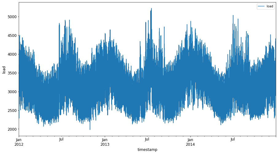

Now, let's build our SVR model.

Create Training and Testing Datasets

Once the data is loaded, separate it into training and testing sets. Reshape the data to create a time-step-based dataset required for SVR. Train the model on the training set, then evaluate its accuracy on the training set, testing set, and the full dataset to assess overall performance. Ensure the test set covers a later time period than the training set to prevent the model from learning future information ² (a phenomenon known as Overfitting).

Assign the two-month period from September 1 to October 31, 2014 to the training set. The test set will include the two-month period from November 1 to December 31, 2014: ²
```
train_start_dt = '2014-11-01 00:00:00'
test_start_dt = '2014-12-30 00:00:00'
```

Visualize the differences: ²

energy[(energy.index < test_start_dt) & (energy.index >= train_start_dt)][['load']].rename(columns={'load':'train'}) \
    .join(energy[test_start_dt:][['load']].rename(columns={'load':'test'}), how='outer') \
    .plot(y=['train', 'test'], figsize=(15, 8), fontsize=12)
plt.xlabel('timestamp', fontsize=12)
plt.ylabel('load', fontsize=12)
plt.show()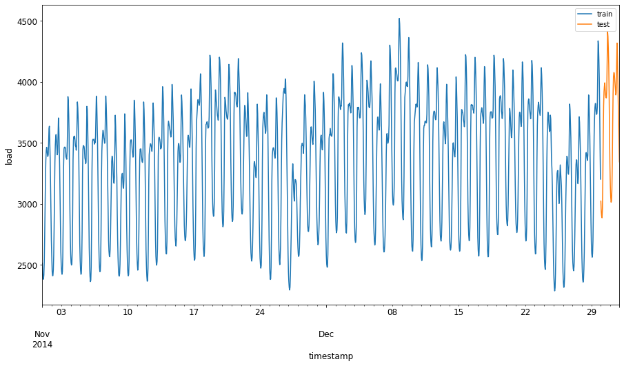

Prepare the Data for Training

Filter and scale the data to prepare it for training. Filter the dataset to include only the required time periods and columns, and scale the data to fit within the range 0 to 1.

Filter the original dataset to include only the specified time periods for each set, and include only the 'load' column and the date: ²

train = energy.copy()[(energy.index >= train_start_dt) & (energy.index < test_start_dt)][['load']]
test = energy.copy()[energy.index >= test_start_dt][['load']]

print('Training data shape: ', train.shape)
print('Test data shape: ', test.shape)

Training data shape:  (1416, 1)
Test data shape:  (48, 1)

Scale the training data to the range (0, 1): ²

scaler = MinMaxScaler()
train['load'] = scaler.fit_transform(train)

Scale the testing data: ²
```
test['load'] = scaler.transform(test)
```

Create Data with Time-Steps ¹

For SVR, transform the input data into the format [batch, timesteps]. Reshape the train_data and test_data to include a new dimension for timesteps.

# Converting to numpy arrays
train_data = train.values
test_data = test.values

For this example, set timesteps = 5. The model's inputs will be data from the first 4 timesteps, and the output will be data from the 5th timestep.

timesteps=5

Convert training data to a 2D tensor using nested list comprehension:

train_data_timesteps=np.array([[j for j in train_data[i:i+timesteps]] for i in range(0,len(train_data)-timesteps+1)])[:,:,0]
train_data_timesteps.shape

(1412, 5)

Convert testing data to a 2D tensor:

test_data_timesteps=np.array([[j for j in test_data[i:i+timesteps]] for i in range(0,len(test_data)-timesteps+1)])[:,:,0]
test_data_timesteps.shape

(44, 5)

Select inputs and outputs from training and testing data:

x_train, y_train = train_data_timesteps[:,:timesteps-1],train_data_timesteps[:,[timesteps-1]]
x_test, y_test = test_data_timesteps[:,:timesteps-1],test_data_timesteps[:,[timesteps-1]]

print(x_train.shape, y_train.shape)
print(x_test.shape, y_test.shape)

(1412, 4) (1412, 1)
(44, 4) (44, 1)

Implement SVR ¹

Now, implement SVR. For more details, refer to this documentation. Follow these steps:

Define the model by calling SVR() and specifying hyperparameters: kernel, gamma, C, and epsilon.
Train the model using the fit() function.
Make predictions using the predict() function.

Create an SVR model using the RBF kernel, with hyperparameters gamma, C, and epsilon set to 0.5, 10, and 0.05, respectively.

model = SVR(kernel='rbf',gamma=0.5, C=10, epsilon = 0.05)

Train the Model on Training Data ¹

model.fit(x_train, y_train[:,0])

SVR(C=10, cache_size=200, coef0=0.0, degree=3, epsilon=0.05, gamma=0.5,
    kernel='rbf', max_iter=-1, shrinking=True, tol=0.001, verbose=False)

Make Model Predictions ¹

y_train_pred = model.predict(x_train).reshape(-1,1)
y_test_pred = model.predict(x_test).reshape(-1,1)

print(y_train_pred.shape, y_test_pred.shape)

(1412, 1) (44, 1)

Your SVR model is ready! Now, let's evaluate it.

Evaluate Your Model ¹

To evaluate the model, first scale the data back to its original range. Then, assess performance by plotting the original and predicted time series and calculating the MAPE.

Scale the predicted and original output:

# Scaling the predictions
y_train_pred = scaler.inverse_transform(y_train_pred)
y_test_pred = scaler.inverse_transform(y_test_pred)

print(len(y_train_pred), len(y_test_pred))

# Scaling the original values
y_train = scaler.inverse_transform(y_train)
y_test = scaler.inverse_transform(y_test)

print(len(y_train), len(y_test))

Evaluate Model Performance on Training and Testing Data ¹

Extract timestamps from the dataset for the x-axis of the plot. Note that the first timesteps-1 values are used as input for the first output, so the timestamps for the output start after that.

train_timestamps = energy[(energy.index < test_start_dt) & (energy.index >= train_start_dt)].index[timesteps-1:]
test_timestamps = energy[test_start_dt:].index[timesteps-1:]

print(len(train_timestamps), len(test_timestamps))

1412 44

Plot predictions for training data:

plt.figure(figsize=(25,6))
plt.plot(train_timestamps, y_train, color = 'red', linewidth=2.0, alpha = 0.6)
plt.plot(train_timestamps, y_train_pred, color = 'blue', linewidth=0.8)
plt.legend(['Actual','Predicted'])
plt.xlabel('Timestamp')
plt.title("Training data prediction")
plt.show()

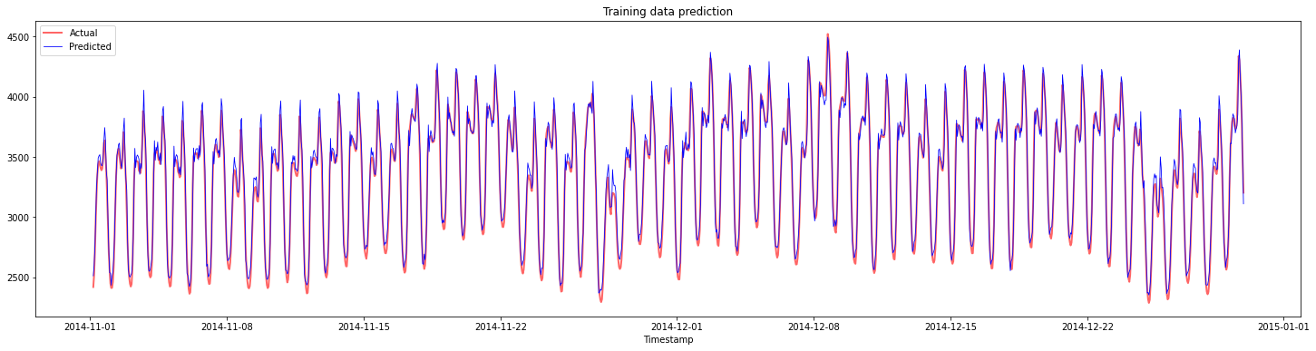
Print MAPE for training data:

print('MAPE for training data: ', mape(y_train_pred, y_train)*100, '%')

MAPE for training data: 1.7195710200875551 %

Plot predictions for testing data:

plt.figure(figsize=(10,3))
plt.plot(test_timestamps, y_test, color = 'red', linewidth=2.0, alpha = 0.6)
plt.plot(test_timestamps, y_test_pred, color = 'blue', linewidth=0.8)
plt.legend(['Actual','Predicted'])
plt.xlabel('Timestamp')
plt.show()

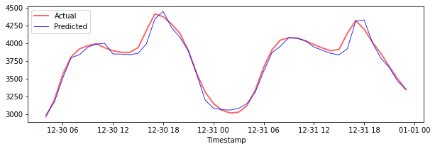
Print MAPE for testing data:

print('MAPE for testing data: ', mape(y_test_pred, y_test)*100, '%')

MAPE for testing data:  1.2623790187854018 %

🏆 Excellent results on the testing dataset!

Evaluate Model Performance on Full Dataset ¹

# Extracting load values as numpy array
data = energy.copy().values

# Scaling
data = scaler.transform(data)

# Transforming to 2D tensor as per model input requirement
data_timesteps=np.array([[j for j in data[i:i+timesteps]] for i in range(0,len(data)-timesteps+1)])[:,:,0]
print("Tensor shape: ", data_timesteps.shape)

# Selecting inputs and outputs from data
X, Y = data_timesteps[:,:timesteps-1],data_timesteps[:,[timesteps-1]]
print("X shape: ", X.shape,"\nY shape: ", Y.shape)

Tensor shape:  (26300, 5)
X shape:  (26300, 4) 
Y shape:  (26300, 1)

# Make model predictions
Y_pred = model.predict(X).reshape(-1,1)

# Inverse scale and reshape
Y_pred = scaler.inverse_transform(Y_pred)
Y = scaler.inverse_transform(Y)

plt.figure(figsize=(30,8))
plt.plot(Y, color = 'red', linewidth=2.0, alpha = 0.6)
plt.plot(Y_pred, color = 'blue', linewidth=0.8)
plt.legend(['Actual','Predicted'])
plt.xlabel('Timestamp')
plt.show()

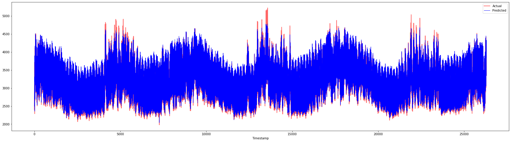
print('MAPE: ', mape(Y_pred, Y)*100, '%')

MAPE:  2.0572089029888656 %

🏆 Great plots, showing a model with strong accuracy. Well done!

🚀Challenge

Experiment with different hyperparameters (gamma, C, epsilon) and evaluate their impact on the testing data. Learn more about these hyperparameters here.
Try different kernel functions and analyze their performance on the dataset. Refer to this document.
Test different values for timesteps to see how the model performs with varying look-back periods.

Post-lecture quiz

Review & Self Study

This lesson introduced SVR for time series forecasting. For more information on SVR, check out this blog. The scikit-learn documentation provides a detailed explanation of SVMs, SVRs, and kernel functions.

Assignment

A new SVR model

Credits

Disclaimer:
This document has been translated using the AI translation service Co-op Translator. While we strive for accuracy, please note that automated translations may contain errors or inaccuracies. The original document in its native language should be regarded as the authoritative source. For critical information, professional human translation is recommended. We are not responsible for any misunderstandings or misinterpretations resulting from the use of this translation.

Text, code, and output in this section contributed by @AnirbanMukherjeeXD ↩︎
Text, code, and output in this section sourced from ARIMA ↩︎