History

leestott fad44a68c4 🌐 Update translations via Co-op Translator		3 weeks ago
..
solution	🌐 Update translations via Co-op Translator	3 weeks ago
working	🌐 Update translations via Co-op Translator	3 weeks ago
README.md	🌐 Update translations via Co-op Translator	3 weeks ago
assignment.md	🌐 Update translations via Co-op Translator	3 weeks ago

Time series forecasting with ARIMA

In the previous lesson, you explored time series forecasting and worked with a dataset showing variations in electrical load over time.

🎥 Click the image above to watch a video: A brief introduction to ARIMA models. The example uses R, but the concepts apply universally.

Introduction

In this lesson, you'll learn how to build models using ARIMA: AutoRegressive Integrated Moving Average. ARIMA models are particularly effective for analyzing data with non-stationarity.

General concepts

To work with ARIMA, you need to understand a few key concepts:

🎓 Stationarity: In statistics, stationarity refers to data whose distribution remains constant over time. Non-stationary data, on the other hand, exhibits trends or fluctuations that need to be transformed for analysis. For example, seasonality can cause fluctuations in data, which can be addressed through 'seasonal differencing.'
🎓 Differencing: Differencing is a statistical technique used to transform non-stationary data into stationary data by removing trends. "Differencing eliminates changes in the level of a time series, removing trends and seasonality, and stabilizing the mean of the time series." Paper by Shixiong et al

ARIMA in the context of time series

Let’s break down the components of ARIMA to understand how it models time series data and enables predictions.

AR - AutoRegressive: Autoregressive models analyze past values (lags) in your data to make predictions. For example, if you have monthly sales data for pencils, each month's sales total is considered an 'evolving variable.' The model is built by regressing the variable of interest on its lagged (previous) values. Wikipedia
I - Integrated: Unlike ARMA models, the 'I' in ARIMA refers to its integrated aspect. Integration involves applying differencing steps to eliminate non-stationarity.
MA - Moving Average: The moving-average component of the model uses current and past values of lags to determine the output variable.

In summary, ARIMA is designed to fit time series data as closely as possible for effective modeling and forecasting.

Exercise - Build an ARIMA model

Navigate to the /working folder in this lesson and locate the notebook.ipynb file.

Run the notebook to load the statsmodels Python library, which is required for ARIMA models.
Import the necessary libraries.

Next, load additional libraries for data visualization:

import os
import warnings
import matplotlib.pyplot as plt
import numpy as np
import pandas as pd
import datetime as dt
import math

from pandas.plotting import autocorrelation_plot
from statsmodels.tsa.statespace.sarimax import SARIMAX
from sklearn.preprocessing import MinMaxScaler
from common.utils import load_data, mape
from IPython.display import Image

%matplotlib inline
pd.options.display.float_format = '{:,.2f}'.format
np.set_printoptions(precision=2)
warnings.filterwarnings("ignore") # specify to ignore warning messages

Load the data from the /data/energy.csv file into a Pandas dataframe and inspect it:
```
energy = load_data('./data')[['load']]
energy.head(10)
```

Plot the energy data from January 2012 to December 2014. This data should look familiar from the previous lesson:

energy.plot(y='load', subplots=True, figsize=(15, 8), fontsize=12)
plt.xlabel('timestamp', fontsize=12)
plt.ylabel('load', fontsize=12)
plt.show()

Now, let’s build a model!

Create training and testing datasets

After loading the data, split it into training and testing sets. The model will be trained on the training set and evaluated for accuracy using the testing set. Ensure the testing set covers a later time period than the training set to avoid data leakage.

Assign the period from September 1 to October 31, 2014 to the training set. The testing set will cover November 1 to December 31, 2014:
```
train_start_dt = '2014-11-01 00:00:00'
test_start_dt = '2014-12-30 00:00:00'
```
Since the data represents daily energy consumption, it exhibits a strong seasonal pattern, but recent days' consumption is most similar to current consumption.

Visualize the differences:

energy[(energy.index < test_start_dt) & (energy.index >= train_start_dt)][['load']].rename(columns={'load':'train'}) \
    .join(energy[test_start_dt:][['load']].rename(columns={'load':'test'}), how='outer') \
    .plot(y=['train', 'test'], figsize=(15, 8), fontsize=12)
plt.xlabel('timestamp', fontsize=12)
plt.ylabel('load', fontsize=12)
plt.show()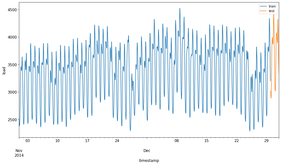

Using a relatively small training window should suffice.

Note: The function used to fit the ARIMA model performs in-sample validation during fitting, so validation data is omitted.

Prepare the data for training

Prepare the data for training by filtering and scaling it. Filter the dataset to include only the required time periods and columns, and scale the data to fit within the range 0 to 1.

Filter the dataset to include only the specified time periods and the 'load' column along with the date:

train = energy.copy()[(energy.index >= train_start_dt) & (energy.index < test_start_dt)][['load']]
test = energy.copy()[energy.index >= test_start_dt][['load']]

print('Training data shape: ', train.shape)
print('Test data shape: ', test.shape)

Check the shape of the filtered data:

Training data shape:  (1416, 1)
Test data shape:  (48, 1)

Scale the data to fit within the range (0, 1):

scaler = MinMaxScaler()
train['load'] = scaler.fit_transform(train)
train.head(10)

Compare the original data to the scaled data:

energy[(energy.index >= train_start_dt) & (energy.index < test_start_dt)][['load']].rename(columns={'load':'original load'}).plot.hist(bins=100, fontsize=12)
train.rename(columns={'load':'scaled load'}).plot.hist(bins=100, fontsize=12)
plt.show()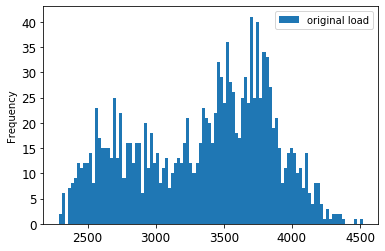

The original data

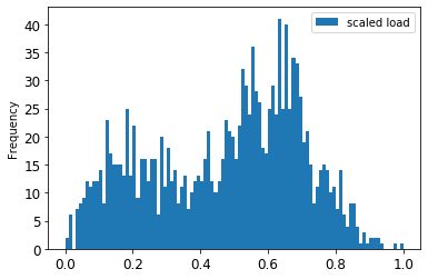
The scaled data

Scale the test data using the same approach:

test['load'] = scaler.transform(test)
test.head()

Implement ARIMA

Now it’s time to implement ARIMA using the statsmodels library.

Follow these steps:

Define the model by calling SARIMAX() and specifying the model parameters: p, d, q, and P, D, Q.
Train the model on the training data using the fit() function.
Make predictions using the forecast() function, specifying the number of steps (the horizon) to forecast.

🎓 What do these parameters mean? ARIMA models use three parameters to capture key aspects of time series data: seasonality, trend, and noise.

p: Represents the auto-regressive component, incorporating past values. d: Represents the integrated component, determining the level of differencing to apply. q: Represents the moving-average component.

Note: For seasonal data (like this dataset), use a seasonal ARIMA model (SARIMA) with additional parameters: P, D, and Q, which correspond to the seasonal components of p, d, and q.

Set the horizon value to 3 hours:
```
# Specify the number of steps to forecast ahead
HORIZON = 3
print('Forecasting horizon:', HORIZON, 'hours')
```
Selecting optimal ARIMA parameters can be challenging. Consider using the auto_arima() function from the pyramid library.

For now, manually select parameters to find a suitable model:

order = (4, 1, 0)
seasonal_order = (1, 1, 0, 24)

model = SARIMAX(endog=train, order=order, seasonal_order=seasonal_order)
results = model.fit()

print(results.summary())

A table of results is displayed.

Congratulations! You’ve built your first model. Next, evaluate its performance.

Evaluate your model

Evaluate your model using walk forward validation. In practice, time series models are retrained whenever new data becomes available, enabling the best forecast at each time step.

Using this technique:

Train the model on the training set.
Predict the next time step.
Compare the prediction to the actual value.
Expand the training set to include the actual value and repeat the process.

Note: Keep the training set window fixed for efficiency. When adding a new observation to the training set, remove the oldest observation.

This approach provides a robust evaluation of model performance but requires significant computational resources. It’s ideal for small datasets or simple models but may be challenging at scale.

Walk-forward validation is the gold standard for time series model evaluation and is recommended for your projects.

Create a test data point for each HORIZON step:

test_shifted = test.copy()

for t in range(1, HORIZON+1):
    test_shifted['load+'+str(t)] = test_shifted['load'].shift(-t, freq='H')

test_shifted = test_shifted.dropna(how='any')
test_shifted.head(5)

		load	load+1	load+2
2014-12-30	00:00:00	0.33	0.29	0.27
2014-12-30	01:00:00	0.29	0.27	0.27
2014-12-30	02:00:00	0.27	0.27	0.30
2014-12-30	03:00:00	0.27	0.30	0.41
2014-12-30	04:00:00	0.30	0.41	0.57

The data shifts horizontally based on the horizon point.

Use a sliding window approach to make predictions on the test data in a loop:

%%time
training_window = 720 # dedicate 30 days (720 hours) for training

train_ts = train['load']
test_ts = test_shifted

history = [x for x in train_ts]
history = history[(-training_window):]

predictions = list()

order = (2, 1, 0)
seasonal_order = (1, 1, 0, 24)

for t in range(test_ts.shape[0]):
    model = SARIMAX(endog=history, order=order, seasonal_order=seasonal_order)
    model_fit = model.fit()
    yhat = model_fit.forecast(steps = HORIZON)
    predictions.append(yhat)
    obs = list(test_ts.iloc[t])
    # move the training window
    history.append(obs[0])
    history.pop(0)
    print(test_ts.index[t])
    print(t+1, ': predicted =', yhat, 'expected =', obs)

Observe the training process:

2014-12-30 00:00:00
1 : predicted = [0.32 0.29 0.28] expected = [0.32945389435989236, 0.2900626678603402, 0.2739480752014323]

2014-12-30 01:00:00
2 : predicted = [0.3  0.29 0.3 ] expected = [0.2900626678603402, 0.2739480752014323, 0.26812891674127126]

2014-12-30 02:00:00
3 : predicted = [0.27 0.28 0.32] expected = [0.2739480752014323, 0.26812891674127126, 0.3025962399283795]

Compare predictions to actual load values:

eval_df = pd.DataFrame(predictions, columns=['t+'+str(t) for t in range(1, HORIZON+1)])
eval_df['timestamp'] = test.index[0:len(test.index)-HORIZON+1]
eval_df = pd.melt(eval_df, id_vars='timestamp', value_name='prediction', var_name='h')
eval_df['actual'] = np.array(np.transpose(test_ts)).ravel()
eval_df[['prediction', 'actual']] = scaler.inverse_transform(eval_df[['prediction', 'actual']])
eval_df.head()

Output:

		timestamp	h	prediction	actual
0	2014-12-30	00:00:00	t+1	3,008.74	3,023.00
1	2014-12-30	01:00:00	t+1	2,955.53	2,935.00
2	2014-12-30	02:00:00	t+1	2,900.17	2,899.00
3	2014-12-30	03:00:00	t+1	2,917.69	2,886.00
4	2014-12-30	04:00:00	t+1	2,946.99	2,963.00

Examine the hourly predictions compared to actual load values. How accurate are they?

Check model accuracy

Assess your model’s accuracy by calculating its mean absolute percentage error (MAPE) across all predictions. and predicted values is divided by the actual value. "The absolute value in this calculation is summed for every forecasted point in time and divided by the number of fitted points n." wikipedia

Express the equation in code:

if(HORIZON > 1):
    eval_df['APE'] = (eval_df['prediction'] - eval_df['actual']).abs() / eval_df['actual']
    print(eval_df.groupby('h')['APE'].mean())

Calculate the MAPE for one step:

print('One step forecast MAPE: ', (mape(eval_df[eval_df['h'] == 't+1']['prediction'], eval_df[eval_df['h'] == 't+1']['actual']))*100, '%')

One-step forecast MAPE: 0.5570581332313952 %

Print the MAPE for the multi-step forecast:

print('Multi-step forecast MAPE: ', mape(eval_df['prediction'], eval_df['actual'])*100, '%')

Multi-step forecast MAPE:  1.1460048657704118 %

A lower number is better: keep in mind that a forecast with a MAPE of 10 means it's off by 10%.

However, as always, it's easier to understand this kind of accuracy measurement visually, so let's plot it:

 if(HORIZON == 1):
    ## Plotting single step forecast
    eval_df.plot(x='timestamp', y=['actual', 'prediction'], style=['r', 'b'], figsize=(15, 8))

else:
    ## Plotting multi step forecast
    plot_df = eval_df[(eval_df.h=='t+1')][['timestamp', 'actual']]
    for t in range(1, HORIZON+1):
        plot_df['t+'+str(t)] = eval_df[(eval_df.h=='t+'+str(t))]['prediction'].values

    fig = plt.figure(figsize=(15, 8))
    ax = plt.plot(plot_df['timestamp'], plot_df['actual'], color='red', linewidth=4.0)
    ax = fig.add_subplot(111)
    for t in range(1, HORIZON+1):
        x = plot_df['timestamp'][(t-1):]
        y = plot_df['t+'+str(t)][0:len(x)]
        ax.plot(x, y, color='blue', linewidth=4*math.pow(.9,t), alpha=math.pow(0.8,t))

    ax.legend(loc='best')

plt.xlabel('timestamp', fontsize=12)
plt.ylabel('load', fontsize=12)
plt.show()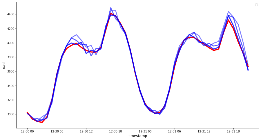

🏆 A very nice plot, showing a model with good accuracy. Well done!

🚀Challenge

Explore different ways to test the accuracy of a Time Series Model. In this lesson, we covered MAPE, but are there other methods you could use? Research them and make notes. A helpful document can be found here

Post-lecture quiz

Review & Self Study

This lesson only introduces the basics of Time Series Forecasting with ARIMA. Take some time to expand your knowledge by exploring this repository and its various model types to learn other approaches to building Time Series models.

Assignment

A new ARIMA model

Disclaimer:
This document has been translated using the AI translation service Co-op Translator. While we aim for accuracy, please note that automated translations may include errors or inaccuracies. The original document in its native language should be regarded as the authoritative source. For critical information, professional human translation is advised. We are not responsible for any misunderstandings or misinterpretations resulting from the use of this translation.

README.md

Unescape Escape

Time series forecasting with ARIMA

Pre-lecture quiz

Introduction

General concepts

ARIMA in the context of time series

Exercise - Build an ARIMA model

Create training and testing datasets

Prepare the data for training

Implement ARIMA

Evaluate your model

Check model accuracy

🚀Challenge

Post-lecture quiz

Review & Self Study

Assignment

README.md Unescape Escape

Time series forecasting with ARIMA

Pre-lecture quiz

Introduction

General concepts

ARIMA in the context of time series

Exercise - Build an ARIMA model

Create training and testing datasets

Prepare the data for training

Implement ARIMA

Evaluate your model

Check model accuracy

🚀Challenge

Post-lecture quiz

Review & Self Study

Assignment

README.md

Unescape Escape