|
|
3 weeks ago | |
|---|---|---|
| .. | ||
| solution | 3 weeks ago | |
| working | 3 weeks ago | |
| README.md | 3 weeks ago | |
| assignment.md | 3 weeks ago | |
README.md
Introduction to time series forecasting
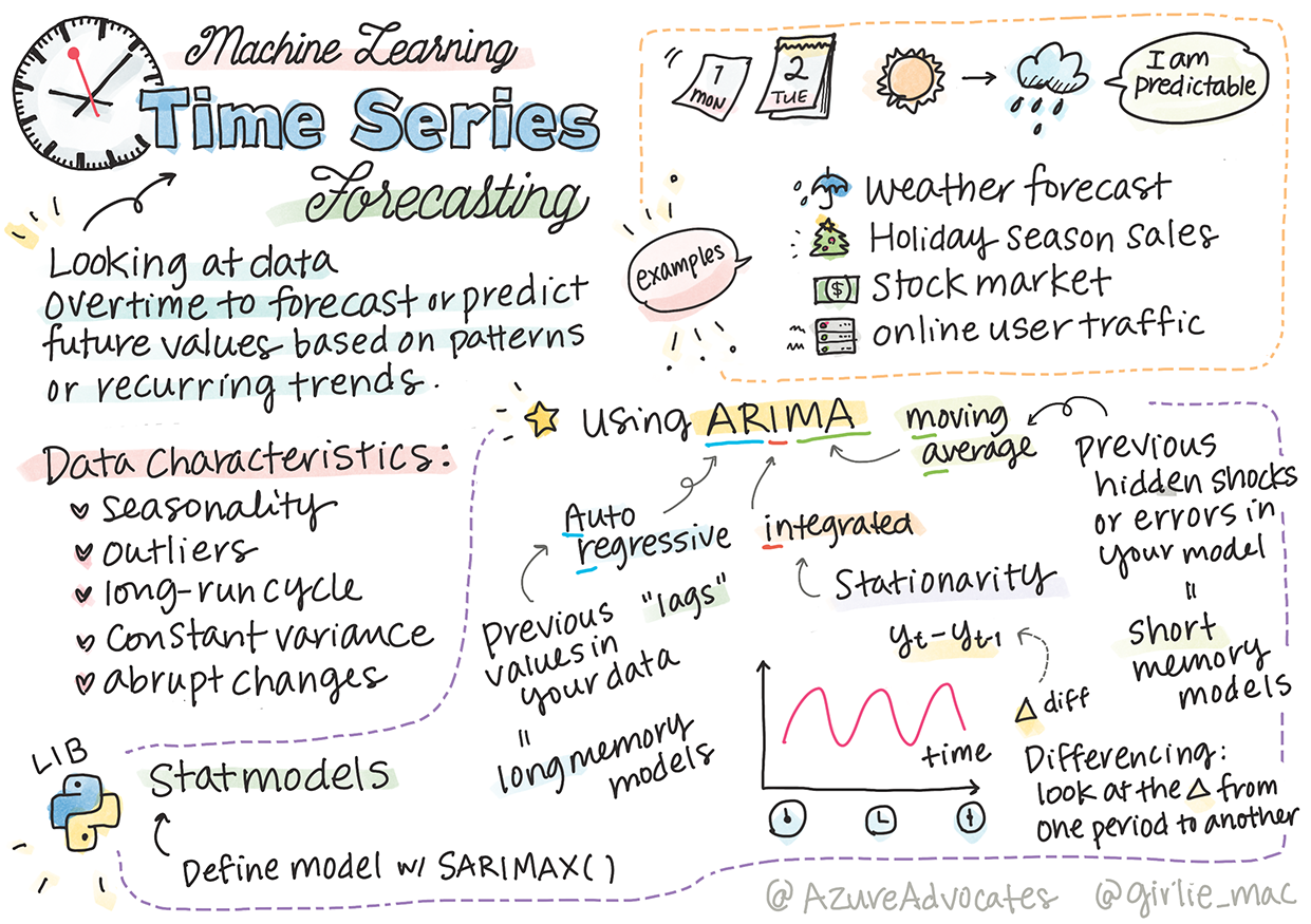
Sketchnote by Tomomi Imura
In this lesson and the next, you'll learn about time series forecasting, an intriguing and valuable skill for machine learning scientists that is less commonly discussed compared to other topics. Time series forecasting is like a "crystal ball": by analyzing past behavior of a variable, such as price, you can predict its potential future value.
🎥 Click the image above to watch a video about time series forecasting
Pre-lecture quiz
This field is both fascinating and practical, offering significant value to businesses due to its direct applications in pricing, inventory management, and supply chain optimization. While deep learning techniques are increasingly being used to improve predictions, time series forecasting remains heavily influenced by traditional machine learning methods.
Penn State offers a helpful time series curriculum here
Introduction
Imagine you manage a network of smart parking meters that collect data on usage frequency and duration over time.
What if you could predict the future value of a meter based on its past performance, using principles of supply and demand?
Forecasting the right time to act in order to achieve your goals is a challenge that time series forecasting can address. While charging more during peak times might not make people happy, it could be an effective way to generate revenue for street maintenance!
Let's dive into some types of time series algorithms and start working with a notebook to clean and prepare data. The dataset you'll analyze comes from the GEFCom2014 forecasting competition. It includes three years of hourly electricity load and temperature data from 2012 to 2014. Using historical patterns in electricity load and temperature, you can predict future electricity load values.
In this example, you'll learn how to forecast one time step ahead using only historical load data. But before we begin, it's important to understand the underlying concepts.
Some definitions
When you encounter the term "time series," it's important to understand its use in various contexts.
🎓 Time series
In mathematics, "a time series is a series of data points indexed (or listed or graphed) in time order. Most commonly, a time series is a sequence taken at successive equally spaced points in time." An example of a time series is the daily closing value of the Dow Jones Industrial Average. Time series plots and statistical modeling are often used in signal processing, weather forecasting, earthquake prediction, and other fields where events occur and data points can be tracked over time.
🎓 Time series analysis
Time series analysis involves examining the time series data mentioned above. This data can take various forms, including "interrupted time series," which identifies patterns before and after a disruptive event. The type of analysis depends on the nature of the data, which can consist of numbers or characters.
The analysis employs various methods, such as frequency-domain and time-domain approaches, linear and nonlinear techniques, and more. Learn more about the different ways to analyze this type of data.
🎓 Time series forecasting
Time series forecasting uses a model to predict future values based on patterns observed in past data. While regression models can be used to explore time series data, with time indices as x variables on a plot, specialized models are better suited for this type of analysis.
Time series data consists of ordered observations, unlike data analyzed through linear regression. The most common model is ARIMA, which stands for "Autoregressive Integrated Moving Average."
ARIMA models "relate the present value of a series to past values and past prediction errors." These models are particularly useful for analyzing time-domain data, where observations are ordered chronologically.
There are several types of ARIMA models, which you can explore here and will learn about in the next lesson.
In the next lesson, you'll build an ARIMA model using Univariate Time Series, which focuses on a single variable that changes over time. An example of this type of data is this dataset that records monthly CO2 concentrations at the Mauna Loa Observatory:
| CO2 | YearMonth | Year | Month |
|---|---|---|---|
| 330.62 | 1975.04 | 1975 | 1 |
| 331.40 | 1975.13 | 1975 | 2 |
| 331.87 | 1975.21 | 1975 | 3 |
| 333.18 | 1975.29 | 1975 | 4 |
| 333.92 | 1975.38 | 1975 | 5 |
| 333.43 | 1975.46 | 1975 | 6 |
| 331.85 | 1975.54 | 1975 | 7 |
| 330.01 | 1975.63 | 1975 | 8 |
| 328.51 | 1975.71 | 1975 | 9 |
| 328.41 | 1975.79 | 1975 | 10 |
| 329.25 | 1975.88 | 1975 | 11 |
| 330.97 | 1975.96 | 1975 | 12 |
✅ Identify the variable that changes over time in this dataset.
Time Series data characteristics to consider
When analyzing time series data, you may notice certain characteristics that need to be addressed to better understand its patterns. If you think of time series data as providing a "signal" you want to analyze, these characteristics can be considered "noise." You'll often need to reduce this "noise" using statistical techniques.
Here are some key concepts to understand when working with time series data:
🎓 Trends
Trends refer to measurable increases or decreases over time. Read more about how to identify and, if necessary, remove trends from your time series.
Seasonality refers to periodic fluctuations, such as holiday sales spikes. Learn more about how different types of plots reveal seasonality in data.
🎓 Outliers
Outliers are data points that deviate significantly from the standard variance.
🎓 Long-run cycle
Independent of seasonality, data may exhibit long-term cycles, such as economic downturns lasting over a year.
🎓 Constant variance
Some data show consistent fluctuations over time, like daily and nightly energy usage.
🎓 Abrupt changes
Data may display sudden changes that require further analysis. For example, the abrupt closure of businesses due to COVID caused significant shifts in data.
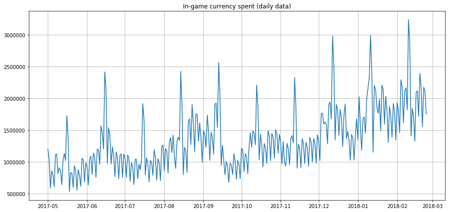
✅ Here's a sample time series plot showing daily in-game currency spent over several years. Can you identify any of the characteristics listed above in this data?
Exercise - getting started with power usage data
Let's begin creating a time series model to predict future power usage based on past usage.
The data in this example comes from the GEFCom2014 forecasting competition. It includes three years of hourly electricity load and temperature data from 2012 to 2014.
Tao Hong, Pierre Pinson, Shu Fan, Hamidreza Zareipour, Alberto Troccoli, and Rob J. Hyndman, "Probabilistic energy forecasting: Global Energy Forecasting Competition 2014 and beyond," International Journal of Forecasting, vol.32, no.3, pp 896-913, July-September, 2016.
-
In the
workingfolder of this lesson, open the notebook.ipynb file. Start by adding libraries to load and visualize data:import os import matplotlib.pyplot as plt from common.utils import load_data %matplotlib inlineNote: You're using files from the included
commonfolder, which sets up your environment and handles data downloading. -
Next, examine the data as a dataframe by calling
load_data()andhead():data_dir = './data' energy = load_data(data_dir)[['load']] energy.head()You'll see two columns representing date and load:
load 2012-01-01 00:00:00 2698.0 2012-01-01 01:00:00 2558.0 2012-01-01 02:00:00 2444.0 2012-01-01 03:00:00 2402.0 2012-01-01 04:00:00 2403.0 -
Now, plot the data by calling
plot():energy.plot(y='load', subplots=True, figsize=(15, 8), fontsize=12) plt.xlabel('timestamp', fontsize=12) plt.ylabel('load', fontsize=12) plt.show()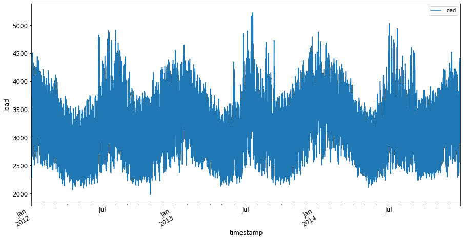
-
Next, plot the first week of July 2014 by providing the date range as input to
energyin[from date]: [to date]format:energy['2014-07-01':'2014-07-07'].plot(y='load', subplots=True, figsize=(15, 8), fontsize=12) plt.xlabel('timestamp', fontsize=12) plt.ylabel('load', fontsize=12) plt.show()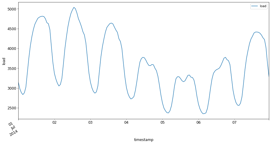
A beautiful plot! Examine these plots and see if you can identify any of the characteristics listed above. What insights can you gather by visualizing the data?
In the next lesson, you'll create an ARIMA model to generate forecasts.
🚀Challenge
Make a list of industries and fields that could benefit from time series forecasting. Can you think of applications in the arts? Econometrics? Ecology? Retail? Industry? Finance? What other areas?
Post-lecture quiz
Review & Self Study
Although not covered here, neural networks are sometimes used to enhance traditional time series forecasting methods. Read more about them in this article.
Assignment
Visualize additional time series
Disclaimer:
This document has been translated using the AI translation service Co-op Translator. While we strive for accuracy, please note that automated translations may contain errors or inaccuracies. The original document in its native language should be regarded as the authoritative source. For critical information, professional human translation is recommended. We are not responsible for any misunderstandings or misinterpretations resulting from the use of this translation.