|
|
3 weeks ago | |
|---|---|---|
| .. | ||
| solution | 3 weeks ago | |
| README.md | 3 weeks ago | |
| assignment.md | 3 weeks ago | |
| notebook.ipynb | 3 weeks ago | |
README.md
Introduction to classification
In these four lessons, you will dive into one of the core areas of traditional machine learning: classification. We'll explore various classification algorithms using a dataset about the diverse and delicious cuisines of Asia and India. Get ready to whet your appetite!

Celebrate pan-Asian cuisines in these lessons! Image by Jen Looper
Classification is a type of supervised learning that shares many similarities with regression techniques. Machine learning is all about predicting values or assigning labels to data using datasets, and classification typically falls into two categories: binary classification and multiclass classification.

🎥 Click the image above for a video: MIT's John Guttag introduces classification
Key points to remember:
- Linear regression helps predict relationships between variables and make accurate predictions about where a new data point might fall relative to a line. For example, you could predict the price of a pumpkin in September versus December.
- Logistic regression helps identify "binary categories": at a certain price point, is this pumpkin orange or not-orange?
Classification uses different algorithms to determine how to assign a label or class to a data point. In this lesson, we'll use cuisine data to see if we can predict the cuisine of origin based on a set of ingredients.
Pre-lecture quiz
This lesson is available in R!
Introduction
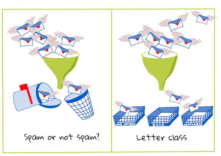
Classification is a fundamental task for machine learning researchers and data scientists. From simple binary classification ("is this email spam or not?") to complex image classification and segmentation using computer vision, the ability to sort data into categories and analyze it is invaluable.
To put it more scientifically, classification involves creating a predictive model that maps the relationship between input variables and output variables.
Binary vs. multiclass problems for classification algorithms to handle. Infographic by Jen Looper
Before we start cleaning, visualizing, and preparing our data for machine learning tasks, let's learn about the different ways machine learning can be used to classify data.
Derived from statistics, classification in traditional machine learning uses features like smoker, weight, and age to predict the likelihood of developing a certain disease. As a supervised learning technique similar to regression, classification uses labeled data to train algorithms to classify and predict features (or 'labels') of a dataset and assign them to a group or outcome.
✅ Take a moment to imagine a dataset about cuisines. What could a multiclass model answer? What could a binary model answer? For instance, could you predict whether a given cuisine is likely to use fenugreek? Or, if you were handed a grocery bag containing star anise, artichokes, cauliflower, and horseradish, could you determine if you could make a typical Indian dish?

🎥 Click the image above for a video. The premise of the show 'Chopped' is the 'mystery basket,' where chefs must create dishes using random ingredients. Imagine how helpful a machine learning model could be!
Hello 'classifier'
The question we want to answer with this cuisine dataset is a multiclass question, as we have several possible national cuisines to consider. Given a set of ingredients, which of these classes does the data belong to?
Scikit-learn provides several algorithms for classifying data, depending on the type of problem you're solving. In the next two lessons, you'll explore some of these algorithms.
Exercise - clean and balance your data
Before diving into the project, the first step is to clean and balance your data to achieve better results. Start with the blank notebook.ipynb file in the root of this folder.
The first thing you'll need to install is imblearn. This Scikit-learn package helps balance datasets (you'll learn more about this shortly).
-
Install
imblearnusingpip install:pip install imblearn -
Import the necessary packages to load and visualize your data, and also import
SMOTEfromimblearn.import pandas as pd import matplotlib.pyplot as plt import matplotlib as mpl import numpy as np from imblearn.over_sampling import SMOTEYou're now ready to import the data.
-
Import the data:
df = pd.read_csv('../data/cuisines.csv')Use
read_csv()to load the contents of the cuisines.csv file into the variabledf. -
Check the shape of the data:
df.head()The first five rows look like this:
| | Unnamed: 0 | cuisine | almond | angelica | anise | anise_seed | apple | apple_brandy | apricot | armagnac | ... | whiskey | white_bread | white_wine | whole_grain_wheat_flour | wine | wood | yam | yeast | yogurt | zucchini | | --- | ---------- | ------- | ------ | -------- | ----- | ---------- | ----- | ------------ | ------- | -------- | --- | ------- | ----------- | ---------- | ----------------------- | ---- | ---- | --- | ----- | ------ | -------- | | 0 | 65 | indian | 0 | 0 | 0 | 0 | 0 | 0 | 0 | 0 | ... | 0 | 0 | 0 | 0 | 0 | 0 | 0 | 0 | 0 | 0 | | 1 | 66 | indian | 1 | 0 | 0 | 0 | 0 | 0 | 0 | 0 | ... | 0 | 0 | 0 | 0 | 0 | 0 | 0 | 0 | 0 | 0 | | 2 | 67 | indian | 0 | 0 | 0 | 0 | 0 | 0 | 0 | 0 | ... | 0 | 0 | 0 | 0 | 0 | 0 | 0 | 0 | 0 | 0 | | 3 | 68 | indian | 0 | 0 | 0 | 0 | 0 | 0 | 0 | 0 | ... | 0 | 0 | 0 | 0 | 0 | 0 | 0 | 0 | 0 | 0 | | 4 | 69 | indian | 0 | 0 | 0 | 0 | 0 | 0 | 0 | 0 | ... | 0 | 0 | 0 | 0 | 0 | 0 | 0 | 0 | 1 | 0 | -
Get information about the data using
info():df.info()The output looks like this:
<class 'pandas.core.frame.DataFrame'>
RangeIndex: 2448 entries, 0 to 2447
Columns: 385 entries, Unnamed: 0 to zucchini
dtypes: int64(384), object(1)
memory usage: 7.2+ MB
Exercise - learning about cuisines
Now the fun begins! Let's explore the distribution of data across cuisines.
-
Plot the data as horizontal bars using
barh():df.cuisine.value_counts().plot.barh()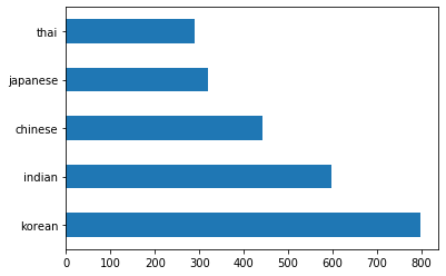
There are a limited number of cuisines, but the data distribution is uneven. You can fix this! Before doing so, let's explore further.
-
Check how much data is available for each cuisine and print the results:
thai_df = df[(df.cuisine == "thai")]
japanese_df = df[(df.cuisine == "japanese")]
chinese_df = df[(df.cuisine == "chinese")]
indian_df = df[(df.cuisine == "indian")]
korean_df = df[(df.cuisine == "korean")]

print(f'thai df: {thai_df.shape}')
print(f'japanese df: {japanese_df.shape}')
print(f'chinese df: {chinese_df.shape}')
print(f'indian df: {indian_df.shape}')
print(f'korean df: {korean_df.shape}')
The output looks like this:
thai df: (289, 385)
japanese df: (320, 385)
chinese df: (442, 385)
indian df: (598, 385)
korean df: (799, 385)
Discovering ingredients
Now let's dig deeper into the data to identify typical ingredients for each cuisine. You'll need to clean out recurring data that might cause confusion between cuisines.
-
Create a Python function
create_ingredient()to generate an ingredient dataframe. This function will drop an unhelpful column and sort ingredients by their count:def create_ingredient_df(df): ingredient_df = df.T.drop(['cuisine','Unnamed: 0']).sum(axis=1).to_frame('value') ingredient_df = ingredient_df[(ingredient_df.T != 0).any()] ingredient_df = ingredient_df.sort_values(by='value', ascending=False, inplace=False) return ingredient_dfUse this function to identify the top ten most popular ingredients for each cuisine.
-
Call
create_ingredient()and plot the results usingbarh():thai_ingredient_df = create_ingredient_df(thai_df) thai_ingredient_df.head(10).plot.barh()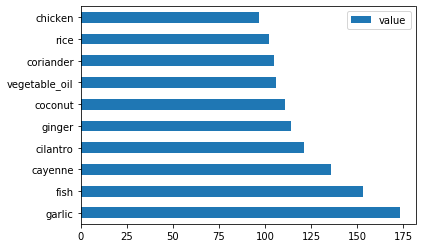
-
Repeat the process for Japanese cuisine:
japanese_ingredient_df = create_ingredient_df(japanese_df)
japanese_ingredient_df.head(10).plot.barh()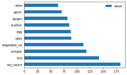
-
Do the same for Chinese cuisine:
chinese_ingredient_df = create_ingredient_df(chinese_df)
chinese_ingredient_df.head(10).plot.barh()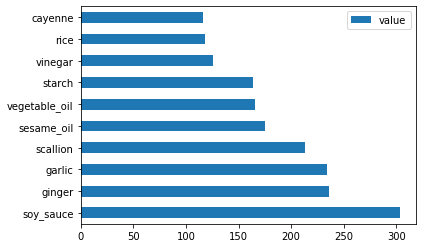
-
Plot the ingredients for Indian cuisine:
indian_ingredient_df = create_ingredient_df(indian_df)
indian_ingredient_df.head(10).plot.barh()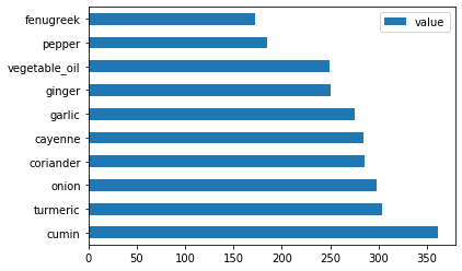
-
Finally, plot the ingredients for Korean cuisine:
korean_ingredient_df = create_ingredient_df(korean_df)
korean_ingredient_df.head(10).plot.barh()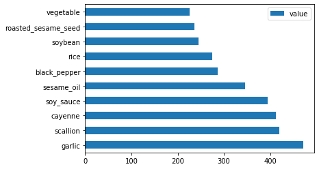
-
Remove common ingredients that might cause confusion between cuisines using
drop():Everyone loves rice, garlic, and ginger!
feature_df= df.drop(['cuisine','Unnamed: 0','rice','garlic','ginger'], axis=1)
labels_df = df.cuisine #.unique()
feature_df.head()
Balance the dataset
Now that the data is cleaned, use SMOTE - "Synthetic Minority Over-sampling Technique" - to balance it.
-
Use
fit_resample()to generate new samples through interpolation.oversample = SMOTE() transformed_feature_df, transformed_label_df = oversample.fit_resample(feature_df, labels_df)Balancing your data improves classification results. For example, in binary classification, if most of your data belongs to one class, the model will predict that class more often simply because there's more data for it. Balancing the data reduces this bias.
-
Check the number of labels per ingredient:
print(f'new label count: {transformed_label_df.value_counts()}')
print(f'old label count: {df.cuisine.value_counts()}')
The output looks like this:
new label count: korean      799
chinese     799
indian      799
japanese    799
thai        799
Name: cuisine, dtype: int64
old label count: korean      799
indian      598
chinese     442
japanese    320
thai        289
Name: cuisine, dtype: int64
The data is now clean, balanced, and ready for analysis!
-
Save the balanced data, including labels and features, into a new dataframe for export:
transformed_df = pd.concat([transformed_label_df,transformed_feature_df],axis=1, join='outer') -
Take one last look at the data using
transformed_df.head()andtransformed_df.info(). Save a copy of this data for use in future lessons:transformed_df.head() transformed_df.info() transformed_df.to_csv("../data/cleaned_cuisines.csv")The new CSV file is now available in the root data folder.
🚀Challenge
This curriculum includes several interesting datasets. Explore the data folders to find datasets suitable for binary or multiclass classification. What questions could you ask of these datasets?
Post-lecture quiz
Review & Self Study
Learn more about SMOTE's API. What use cases is it best suited for? What problems does it address?
Assignment
Explore classification methods
Disclaimer:
This document has been translated using the AI translation service Co-op Translator. While we aim for accuracy, please note that automated translations may include errors or inaccuracies. The original document in its native language should be regarded as the authoritative source. For critical information, professional human translation is advised. We are not responsible for any misunderstandings or misinterpretations resulting from the use of this translation.