History

localizeflow[bot] 3b2098a6fc chore(i18n): sync translations with latest source changes (chunk 1/1, 9 changes)		3 months ago
..
solution	chore(i18n): sync translations with latest source changes (chunk 1/1, 300 changes)	7 months ago
README.md	chore(i18n): sync translations with latest source changes (chunk 1/1, 9 changes)	3 months ago
assignment.md	chore(i18n): sync translations with latest source changes (chunk 1/1, 300 changes)	7 months ago
notebook.ipynb	🌐 Update translations via Co-op Translator	9 months ago

README.md

Introduction to clustering

Clustering na kain Unsupervised Learning wey dey assume say dataset no get label or say im inputs no match any predefined outputs. E dey use different algorithms take sort through unlabeled data come give groupings based on patterns wey e sabi for the data.

🎥 Click di picture wey dey above for video. As you dey study machine learning with clustering, enjoy some Nigerian Dance Hall tracks - dis na highly rated song from 2014 by PSquare.

Pre-lecture quiz

Introduction

Clustering dey very useful for data exploration. Make we see if e fit help find trends and patterns for how Nigerian people dey consume music.

✅ Take one minute think about wetin you fit use clustering do. For real life, clustering dey happen anytime you get pile of laundry and you need to sort out your family members clothes 🧦👕👖🩲. For data science, clustering dey happen when you dey try analyze user preferences, or determine characteristics for any unlabeled dataset. Clustering, for one way, dey help make sense of chaos, like sock drawer.

🎥 Click di picture wey dey above for video: MIT John Guttag dey introduce clustering

For professional side, clustering fit help determine tins like market segmentation, find which age group dey buy which item. Another use na anomaly detection, maybe to detect fraud from credit card transactions dataset. Or you fit use clustering find tumors inside medical scans batch.

✅ Think small about how clustering fit show for banking, e-commerce, or business setting.

🎓 Interesting, cluster analysis come from Anthropology and Psychology for 1930s. You fit imagine how dem fit use am?

Alternatively, you fit use am group search results - by shopping links, images, or reviews, for example. Clustering dey useful if you get big dataset wey you want reduce and also perform detailed analysis, so you fit use am learn about data before you build other models.

✅ Once your data organize inside clusters, you assign am cluster Id, and dis technique fit help protect privacy for dataset; you fit refer to data point by cluster Id instead of using more sensitive identifiable data. You fit think why e good to use cluster Id instead of other cluster elements to identify am?

Deepen your understanding of clustering techniques for this Learn module

Getting started with clustering

Scikit-learn get plenty methods to do clustering. Di type wey you choose go depend on your use case. According to documentation, each method get different benefits. Here na simple table of methods wey Scikit-learn support plus their correct use cases:

Method name	Use case
K-Means	general purpose, inductive
Affinity propagation	many, uneven clusters, inductive
Mean-shift	many, uneven clusters, inductive
Spectral clustering	few, even clusters, transductive
Ward hierarchical clustering	many, constrained clusters, transductive
Agglomerative clustering	many, constrained, non Euclidean distances, transductive
DBSCAN	non-flat geometry, uneven clusters, transductive
OPTICS	non-flat geometry, uneven clusters with variable density, transductive
Gaussian mixtures	flat geometry, inductive
BIRCH	large dataset with outliers, inductive

🎓 How we take create clusters relate well with how we gather data points inside groups. Make we talk some vocabulary:

🎓 'Transductive' vs. 'inductive'

Transductive inference come from observed training cases wey map to specific test cases. Inductive inference come from training cases wey map to general rules wey na only later e dey apply for test cases.

Example: Imagine dataset wey partly get label. Some tins na 'records', some 'cds', others na blank. Your work na provide labels for blank ones. If you choose inductive approach, you go train model to find 'records' and 'cds', then put those labels for unlabeled data. This one go get wahala if e meet tins wey really be 'cassettes'. Transductive approach go handle this unknown data better as e dey group similar tins together, then assign label to the group. For this case, clusters fit show 'round musical tins' and 'square musical tins'.

🎓 'Non-flat' vs. 'flat' geometry

From mathematical talk, non-flat vs. flat geometry na how we measure distance between points either by 'flat' (Euclidean) or 'non-flat' (non-Euclidean) geometrical ways.

'Flat' here mean Euclidean geometry (like 'plane' geometry), non-flat mean non-Euclidean geometry. Wetin geometry get to do with machine learning? As math dey the root of both, e sure say we need one way to measure distances between points for clusters, and dis fit be 'flat' or 'non-flat' based on data nature. Euclidean distances na length of straight line between two points. Non-Euclidean distances na measurement along curve. If data no dey for plane, you go need special algorithm to handle am.

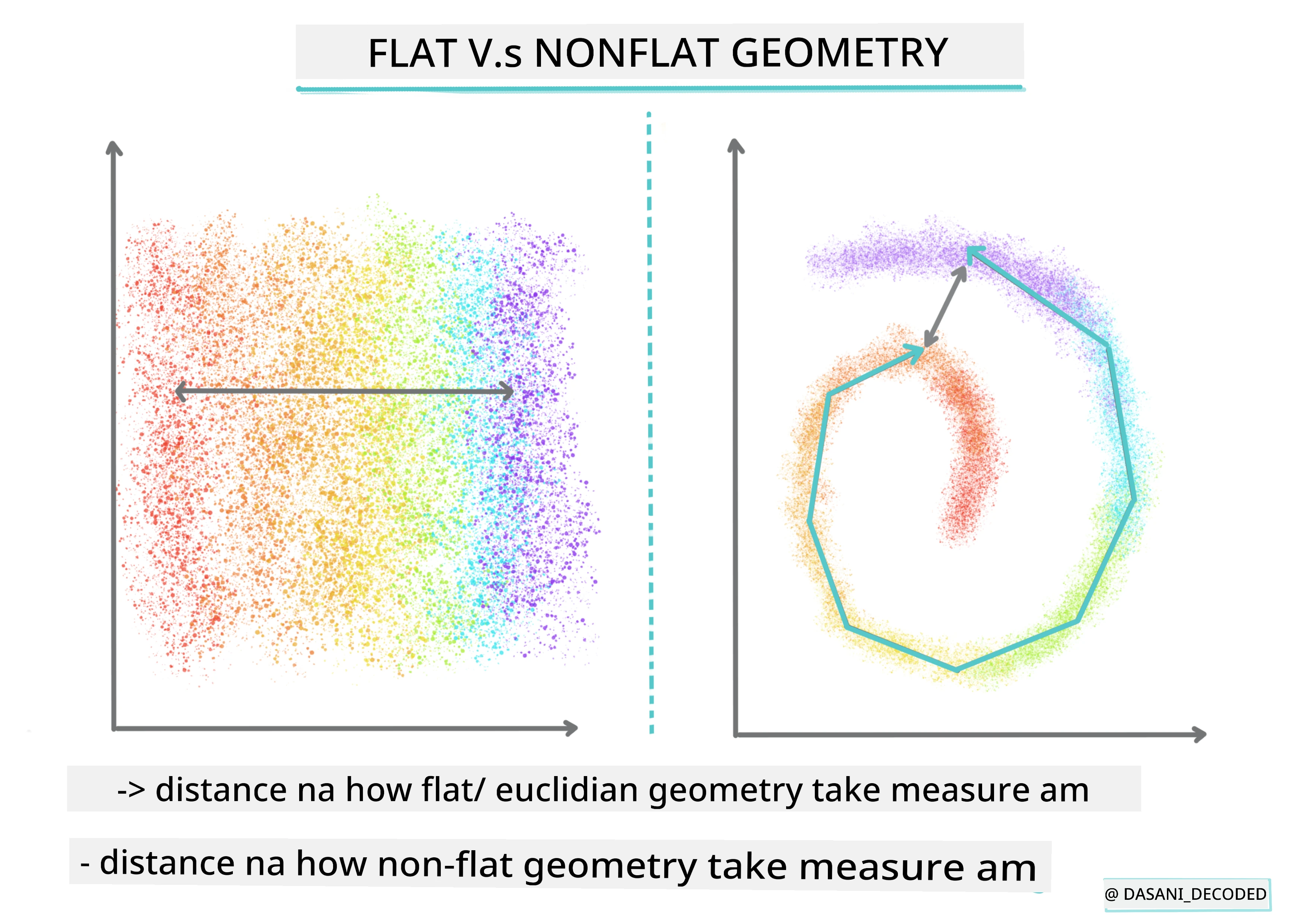
Infographic by Dasani Madipalli

🎓 'Distances'

Clusters dey defined by their distance matrix, like distance between points. You fit measure dis distance in different ways. Euclidean clusters define by average of point values and get 'centroid' or center point. Distances na how far the point dey from that centroid. Non-Euclidean distances na 'clustroids', point wey close to other points. Clustroids fit get different definitions.

🎓 'Constrained'

Constrained Clustering dey add 'semi-supervised' learning inside this unsupervised method. Relationships between points fit get tags like 'cannot link' or 'must-link' so rules go control dataset.

Example: If algorithm loose for batch of unlabelled or semi-labelled data, the clusters e produce fit no dey good quality. For example, clusters fit group 'round music tins', 'square music tins', 'triangular tins', and 'cookies'. If rules dey like ("item must be plastic", "item fit produce music"), e fit help algorithm make better choices.

🎓 'Density'

Data wey noisy dey considered 'dense'. The distances between points for each cluster fit show more or less density, or 'crowded', so data go need the correct clustering method. Dis article show difference between K-Means clustering vs. HDBSCAN algorithms to explore noisy dataset wey get uneven cluster density.

Clustering algorithms

Over 100 clustering algorithms dey, and how you go use dem depend on data nature. Make we yarn some major ones:

Hierarchical clustering. If object classify based on how near e be another object, instead of one far, clusters form based on members distance to and from other objects. Scikit-learn agglomerative clustering na hierarchical.

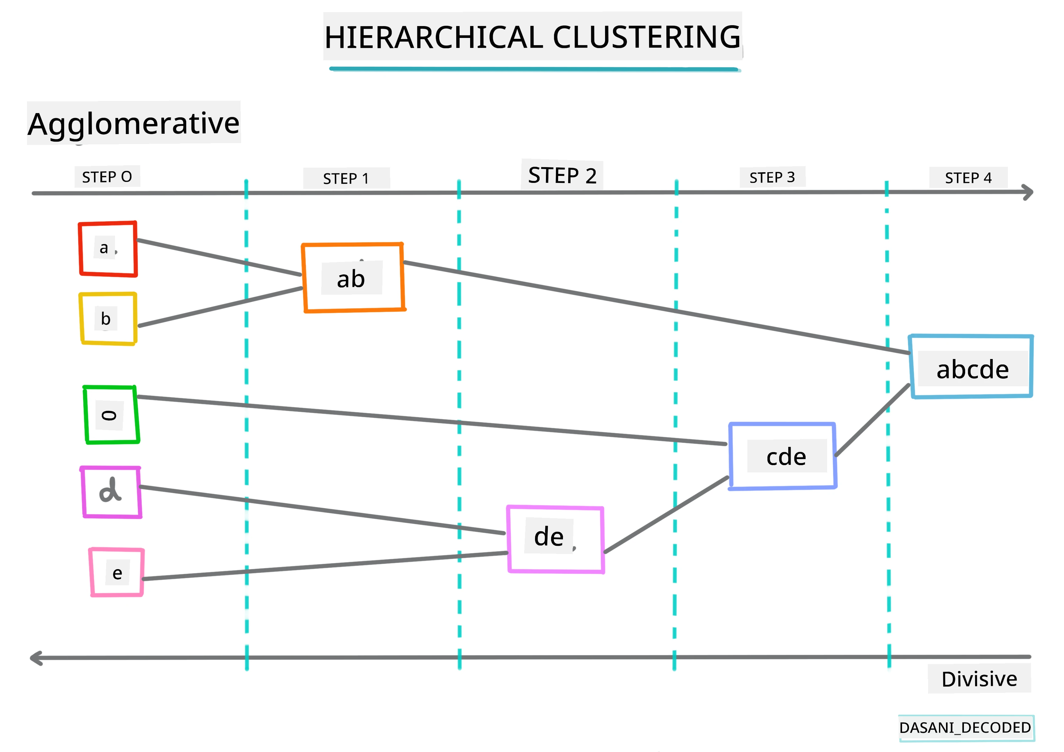
Infographic by Dasani Madipalli
Centroid clustering. Dis popular algorithm need you choose 'k', the number of clusters to form, then e go find center point of cluster and gather data around am. K-means clustering na popular centroid clustering version. Center na nearest mean, so na im get the name. Squared distance from cluster minimise.

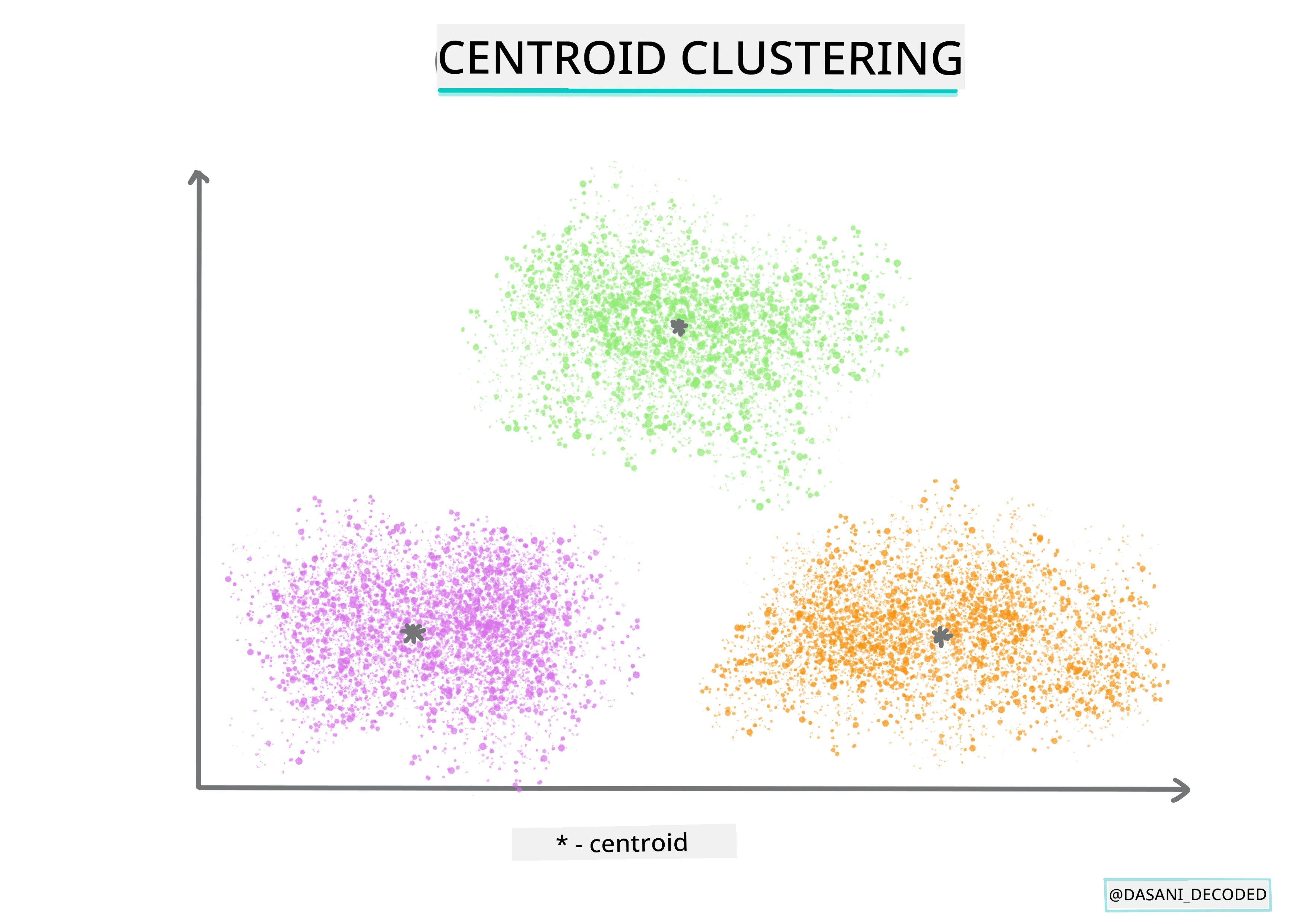
Infographic by Dasani Madipalli
Distribution-based clustering. Based on statistical modeling, distribution-based clustering go fit find probability say data point belong to cluster, then assign am correct. Gaussian mixture methods dey here.
Density-based clustering. Data points assign to clusters based on their density, or how dem group together. Points far from group count as outliers or noise. DBSCAN, Mean-shift and OPTICS na this one.
Grid-based clustering. For multi-dimensional datasets, grid dey created and data divide inside grid cells, create clusters.

Exercise - cluster your data

Clustering as technique dey well supported by good visualization, so make we start by visualizing our music data. Dis exercise go help us decide which clustering method make sense for this data nature.

Open notebook.ipynb file for dis folder.
Import Seaborn package for better data visualization.
```
!pip install seaborn
```

Append song data from nigerian-songs.csv. Load dataframe with some data about di songs. Get ready to explore dis data by importing libraries and dumping out data:

import matplotlib.pyplot as plt
import pandas as pd

df = pd.read_csv("../data/nigerian-songs.csv")
df.head()

Check first few lines of data:

	name	album	artist	artist_top_genre	release_date	length	popularity	danceability	acousticness	energy	instrumentalness	liveness	loudness	speechiness	tempo	time_signature
0	Sparky	Mandy & The Jungle	Cruel Santino	alternative r&b	2019	144000	48	0.666	0.851	0.42	0.534	0.11	-6.699	0.0829	133.015	5
1	shuga rush	EVERYTHING YOU HEARD IS TRUE	Odunsi (The Engine)	afropop	2020	89488	30	0.71	0.0822	0.683	0.000169	0.101	-5.64	0.36	129.993	3
2	LITT!	LITT!	AYLØ	indie r&b	2018	207758	40	0.836	0.272	0.564	0.000537	0.11	-7.127	0.0424	130.005	4
3	Confident / Feeling Cool	Enjoy Your Life	Lady Donli	nigerian pop	2019	175135	14	0.894	0.798	0.611	0.000187	0.0964	-4.961	0.113	111.087	4
4	wanted you	rare.	Odunsi (The Engine)	afropop	2018	152049	25	0.702	0.116	0.833	0.91	0.348	-6.044	0.0447	105.115	4

Mek we find some information about di dataframe, call info():

df.info()

Di output go look like dis:

<class 'pandas.core.frame.DataFrame'>
RangeIndex: 530 entries, 0 to 529
Data columns (total 16 columns):
 #   Column            Non-Null Count  Dtype  
---  ------            --------------  -----  
 0   name              530 non-null    object 
 1   album             530 non-null    object 
 2   artist            530 non-null    object 
 3   artist_top_genre  530 non-null    object 
 4   release_date      530 non-null    int64  
 5   length            530 non-null    int64  
 6   popularity        530 non-null    int64  
 7   danceability      530 non-null    float64
 8   acousticness      530 non-null    float64
 9   energy            530 non-null    float64
 10  instrumentalness  530 non-null    float64
 11  liveness          530 non-null    float64
 12  loudness          530 non-null    float64
 13  speechiness       530 non-null    float64
 14  tempo             530 non-null    float64
 15  time_signature    530 non-null    int64  
dtypes: float64(8), int64(4), object(4)
memory usage: 66.4+ KB

Check well-well for null values, call isnull() then verify say di sum na 0:

df.isnull().sum()

E dey good:

name                0
album               0
artist              0
artist_top_genre    0
release_date        0
length              0
popularity          0
danceability        0
acousticness        0
energy              0
instrumentalness    0
liveness            0
loudness            0
speechiness         0
tempo               0
time_signature      0
dtype: int64

Make we describe di data:

df.describe()

	release_date	length	popularity	danceability	acousticness	energy	instrumentalness	liveness	loudness	speechiness	tempo	time_signature
count	530	530	530	530	530	530	530	530	530	530	530	530
mean	2015.390566	222298.1698	17.507547	0.741619	0.265412	0.760623	0.016305	0.147308	-4.953011	0.130748	116.487864	3.986792
std	3.131688	39696.82226	18.992212	0.117522	0.208342	0.148533	0.090321	0.123588	2.464186	0.092939	23.518601	0.333701
min	1998	89488	0	0.255	0.000665	0.111	0	0.0283	-19.362	0.0278	61.695	3
25%	2014	199305	0	0.681	0.089525	0.669	0	0.07565	-6.29875	0.0591	102.96125	4
50%	2016	218509	13	0.761	0.2205	0.7845	0.000004	0.1035	-4.5585	0.09795	112.7145	4
75%	2017	242098.5	31	0.8295	0.403	0.87575	0.000234	0.164	-3.331	0.177	125.03925	4
max	2020	511738	73	0.966	0.954	0.995	0.91	0.811	0.582	0.514	206.007	5

🤔 If we dey work wit clustering, wey na unsupervised method wey no need labeled data, why this data get labels for dis phase? For data exploration time, dem dey important, but clustering algorithm no need di labels. You fit just remove di column headers den you refer di data by di column number.

Make we look di general values of di data. Note say popularity fit be '0', wey mean say di song no get ranking. Make we remove dem small time.

Use barplot find di most popular genres:

import seaborn as sns

top = df['artist_top_genre'].value_counts()
plt.figure(figsize=(10,7))
sns.barplot(x=top[:5].index,y=top[:5].values)
plt.xticks(rotation=45)
plt.title('Top genres',color = 'blue')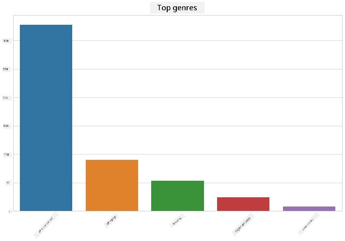

✅ If you want see more top values, change di top [:5] go bigger number, or remove am to see all.

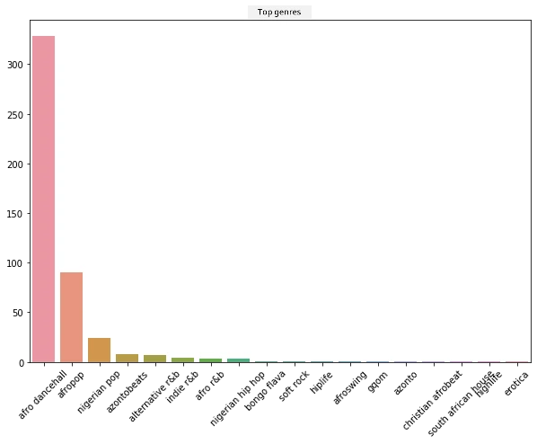
Note, when top genre write as 'Missing', e mean say Spotify no classify am, so make we remove am.

Remove missing data by filtering am out

df = df[df['artist_top_genre'] != 'Missing']
top = df['artist_top_genre'].value_counts()
plt.figure(figsize=(10,7))
sns.barplot(x=top.index,y=top.values)
plt.xticks(rotation=45)
plt.title('Top genres',color = 'blue')

Now check di genres again:

Di top three genres control dis dataset well well. Make we focus on afro dancehall, afropop, and nigerian pop, plus filter di dataset to remove all wey get 0 popularity (meaning dem no get popularity rank for di dataset and fit consider as noise for our work):

df = df[(df['artist_top_genre'] == 'afro dancehall') | (df['artist_top_genre'] == 'afropop') | (df['artist_top_genre'] == 'nigerian pop')]
df = df[(df['popularity'] > 0)]
top = df['artist_top_genre'].value_counts()
plt.figure(figsize=(10,7))
sns.barplot(x=top.index,y=top.values)
plt.xticks(rotation=45)
plt.title('Top genres',color = 'blue')

Do quick test to see if data get strong correlation anywhere:
```
corrmat = df.corr(numeric_only=True)
f, ax = plt.subplots(figsize=(12, 9))
sns.heatmap(corrmat, vmax=.8, square=True)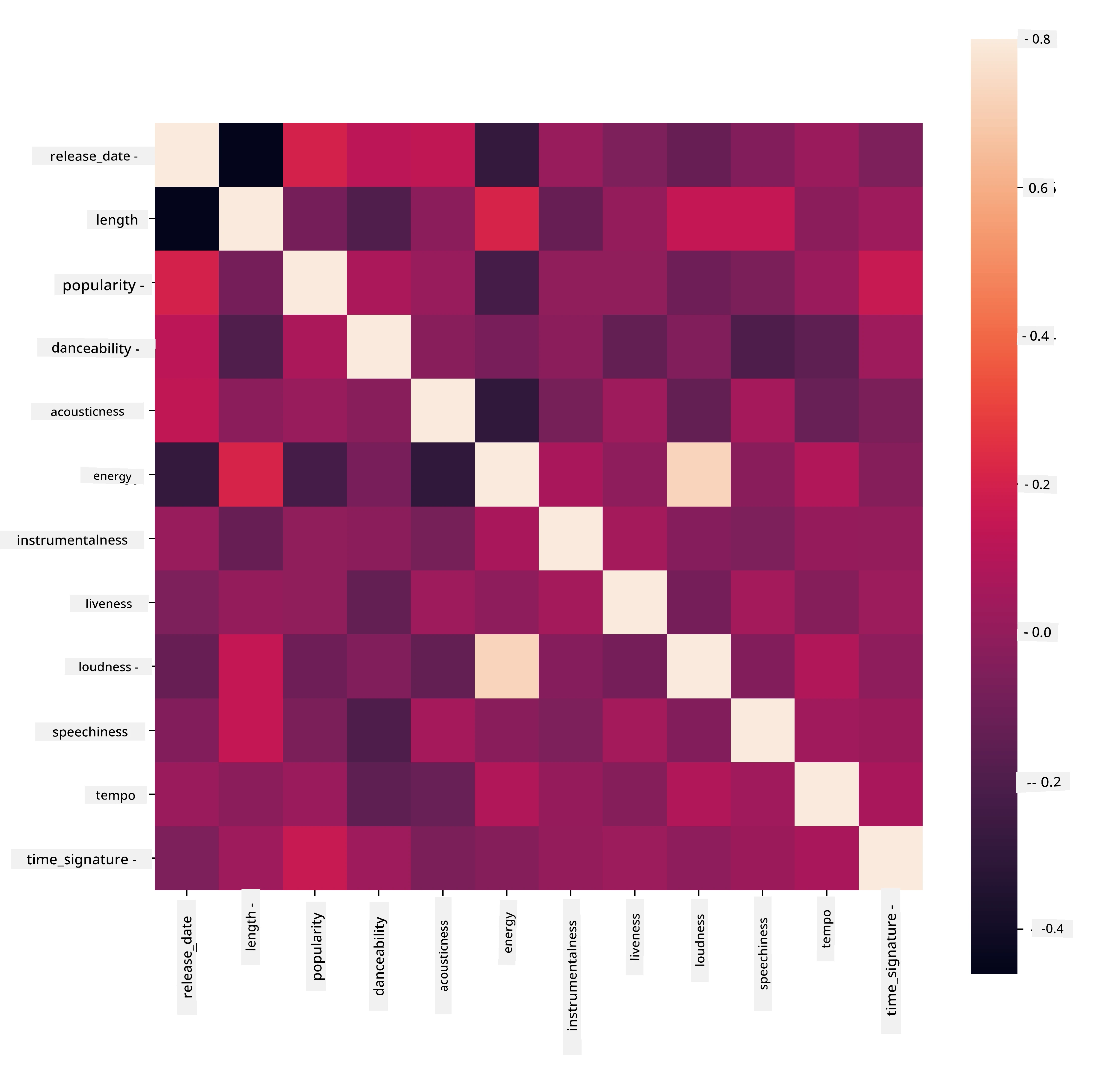
```
Di only strong correlation na between energy and loudness, wey no surprise, becos loud music dey usually get energy. Di other correlations na small small. E go interesting to see wetin clustering algorithm fit do wit dis data.

🎓 Note say correlation no mean causation! We get proof say dem correlate but no proof say one cause the other. One fun website get visuals wey show dis point well.

Di dataset get any pattern wey show say song popularity and danceability dey relate? One FacetGrid dey show say dem get circles wey dey line up well, no matter di genre. E fit be say Nigerian taste dey converge for one level of danceability for dis genre?

✅ Try other datapoints (energy, loudness, speechiness) and different musical genres. Wetin you fit discover? Check df.describe() table to see general data spread.

Exercise - data distribution

These three genres differ well-well in how we dey perceive their danceability, based on their popularity?

Check our top three genres data distribution for popularity and danceability for given x and y axis.
```
sns.set_theme(style="ticks")

g = sns.jointplot(
    data=df,
    x="popularity", y="danceability", hue="artist_top_genre",
    kind="kde",
)
```
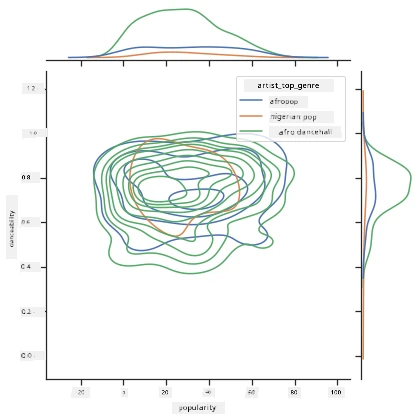
You go fit discover concentric circles around one general convergence point, wey show di distribution.

🎓 Note say dis example dey use KDE (Kernel Density Estimate) graph wey represent data wit continuous probability density curve. E help make sense of multiple distributions.

Generally, di three genres dey loosely align for popularity and danceability. To find clusters for dis loosely-aligned data go be challenge:

Make scatter plot:

sns.FacetGrid(df, hue="artist_top_genre", height=5) \
   .map(plt.scatter, "popularity", "danceability") \
   .add_legend()

Scatterplot of same axes show similar convergence pattern

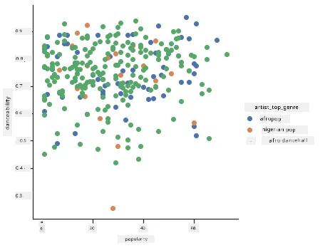
For clustering, you fit use scatterplots show data clusters, so to sabi dis type visualization na important. For next lesson, we go use dis filtered data take k-means clustering find groups wey get interesting overlaps.

🚀Challenge

To prepare for next lesson, make chart about different clustering algorithms wey you fit find and use for production environment. Wetin clustering dey try solve?

Post-lecture quiz

Review & Self Study

Before you begin clustering algorithms, as we don learn, e good make you understand your dataset well-well. Read more on dis topic here

This helpful article go show you different way clustering algorithms dey behave for different data shapes.

Assignment

Research other visualizations for clustering

Disclaimer: Dis document don translate wit AI translation service Co-op Translator. Even tho we dey try make am correct, abeg make you know say automated translation fit get errors or mistakes. Di original document for dia own language na im be di correct source. For important info, make person wey sabi human translation do am. We no go responsible for any misunderstanding or wrong understanding wey fit happen because of dis translation.