# Build a regression model using Scikit-learn: regression four ways
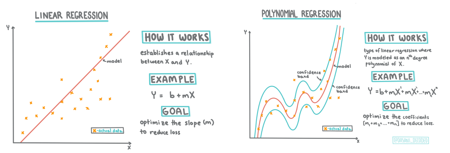
> Infographic by [Dasani Madipalli](https://twitter.com/dasani_decoded)
## [Pre-lecture quiz](https://ff-quizzes.netlify.app/en/ml/)
> ### [This lesson is available in R!](../../../../2-Regression/3-Linear/solution/R/lesson_3.html)
### Introduction
Up to this point, you've explored what regression is using sample data from the pumpkin pricing dataset, which will be used throughout this lesson. You've also visualized the data using Matplotlib.
Now, you're ready to delve deeper into regression for machine learning. While visualization helps you understand the data, the true power of machine learning lies in _training models_. Models are trained on historical data to automatically capture data dependencies, enabling predictions for new data the model hasn't seen before.
In this lesson, you'll learn more about two types of regression: _basic linear regression_ and _polynomial regression_, along with some of the mathematics behind these techniques. These models will help us predict pumpkin prices based on various input data.
[](https://youtu.be/CRxFT8oTDMg "ML for beginners - Understanding Linear Regression")
> 🎥 Click the image above for a short video overview of linear regression.
> Throughout this curriculum, we assume minimal math knowledge and aim to make it accessible for students from other fields. Look out for notes, 🧮 callouts, diagrams, and other tools to aid comprehension.
### Prerequisite
By now, you should be familiar with the structure of the pumpkin dataset we're analyzing. This lesson's _notebook.ipynb_ file contains the preloaded and pre-cleaned data. In the file, pumpkin prices are displayed per bushel in a new data frame. Ensure you can run these notebooks in Visual Studio Code kernels.
### Preparation
As a reminder, you're loading this data to answer specific questions:
- When is the best time to buy pumpkins?
- What price can I expect for a case of miniature pumpkins?
- Should I buy them in half-bushel baskets or 1 1/9 bushel boxes?
Let's continue exploring this data.
In the previous lesson, you created a Pandas data frame and populated it with part of the original dataset, standardizing the pricing by the bushel. However, this only provided about 400 data points, mostly for the fall months.
Take a look at the data preloaded in this lesson's accompanying notebook. The data is preloaded, and an initial scatterplot is charted to show month data. Perhaps we can uncover more details by cleaning the data further.
## A linear regression line
As you learned in Lesson 1, the goal of linear regression is to plot a line that:
- **Shows variable relationships**. Illustrates the relationship between variables.
- **Makes predictions**. Accurately predicts where a new data point would fall relative to the line.
A **Least-Squares Regression** is typically used to draw this type of line. The term 'least-squares' refers to squaring and summing the distances of all data points from the regression line. Ideally, this sum is as small as possible, minimizing errors or `least-squares`.
This approach models a line with the least cumulative distance from all data points. Squaring the terms ensures we're focused on magnitude rather than direction.
> **🧮 Show me the math**
>
> This line, called the _line of best fit_, can be expressed by [an equation](https://en.wikipedia.org/wiki/Simple_linear_regression):
>
> ```
> Y = a + bX
> ```
>
> `X` is the 'explanatory variable', and `Y` is the 'dependent variable'. The slope of the line is `b`, and `a` is the y-intercept, which represents the value of `Y` when `X = 0`.
>
>
>
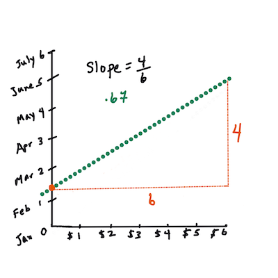
> First, calculate the slope `b`. Infographic by [Jen Looper](https://twitter.com/jenlooper)
>
> For example, in our pumpkin dataset's original question: "predict the price of a pumpkin per bushel by month," `X` would represent the price, and `Y` would represent the month of sale.
>
>
>
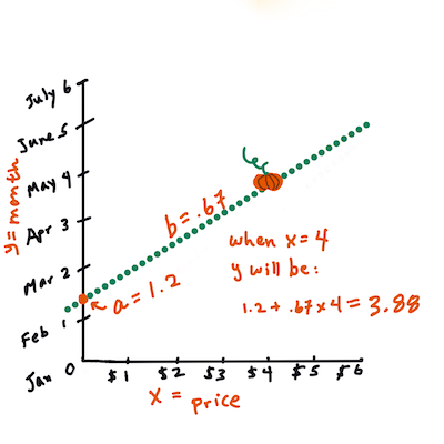
> Calculate the value of Y. If you're paying around $4, it must be April! Infographic by [Jen Looper](https://twitter.com/jenlooper)
>
> The math behind the line calculation demonstrates the slope, which depends on the intercept, or where `Y` is located when `X = 0`.
>
> You can explore the calculation method for these values on the [Math is Fun](https://www.mathsisfun.com/data/least-squares-regression.html) website. Also, check out [this Least-squares calculator](https://www.mathsisfun.com/data/least-squares-calculator.html) to see how the numbers affect the line.
## Correlation
Another important term to understand is the **Correlation Coefficient** between given X and Y variables. Using a scatterplot, you can quickly visualize this coefficient. A plot with data points forming a neat line has high correlation, while a plot with scattered data points has low correlation.
A good linear regression model will have a high (closer to 1 than 0) Correlation Coefficient using the Least-Squares Regression method with a regression line.
✅ Run the notebook accompanying this lesson and examine the Month-to-Price scatterplot. Does the data associating Month to Price for pumpkin sales appear to have high or low correlation based on your visual interpretation of the scatterplot? Does this change if you use a more detailed measure, such as *day of the year* (i.e., the number of days since the start of the year)?
In the code below, we assume the data has been cleaned and a data frame called `new_pumpkins` has been obtained, similar to the following:
ID | Month | DayOfYear | Variety | City | Package | Low Price | High Price | Price
---|-------|-----------|---------|------|---------|-----------|------------|-------
70 | 9 | 267 | PIE TYPE | BALTIMORE | 1 1/9 bushel cartons | 15.0 | 15.0 | 13.636364
71 | 9 | 267 | PIE TYPE | BALTIMORE | 1 1/9 bushel cartons | 18.0 | 18.0 | 16.363636
72 | 10 | 274 | PIE TYPE | BALTIMORE | 1 1/9 bushel cartons | 18.0 | 18.0 | 16.363636
73 | 10 | 274 | PIE TYPE | BALTIMORE | 1 1/9 bushel cartons | 17.0 | 17.0 | 15.454545
74 | 10 | 281 | PIE TYPE | BALTIMORE | 1 1/9 bushel cartons | 15.0 | 15.0 | 13.636364
> The code to clean the data is available in [`notebook.ipynb`](../../../../2-Regression/3-Linear/notebook.ipynb). We performed the same cleaning steps as in the previous lesson and calculated the `DayOfYear` column using the following expression:
```python
day_of_year = pd.to_datetime(pumpkins['Date']).apply(lambda dt: (dt-datetime(dt.year,1,1)).days)
```
Now that you understand the math behind linear regression, let's create a regression model to predict which pumpkin package offers the best prices. This information could be useful for someone buying pumpkins for a holiday pumpkin patch to optimize their purchases.
## Looking for Correlation
[](https://youtu.be/uoRq-lW2eQo "ML for beginners - Looking for Correlation: The Key to Linear Regression")
> 🎥 Click the image above for a short video overview of correlation.
From the previous lesson, you've likely observed that the average price for different months looks like this:
 This suggests there might be some correlation, and we can attempt to train a linear regression model to predict the relationship between `Month` and `Price`, or between `DayOfYear` and `Price`. Here's the scatterplot showing the latter relationship:
 Let's check for correlation using the `corr` function:
```python
print(new_pumpkins['Month'].corr(new_pumpkins['Price']))
print(new_pumpkins['DayOfYear'].corr(new_pumpkins['Price']))
```
The correlation appears to be quite small: -0.15 for `Month` and -0.17 for `DayOfYear`. However, there might be another significant relationship. It seems there are distinct price clusters corresponding to different pumpkin varieties. To confirm this hypothesis, let's plot each pumpkin category using a different color. By passing an `ax` parameter to the `scatter` plotting function, we can plot all points on the same graph:
```python
ax=None
colors = ['red','blue','green','yellow']
for i,var in enumerate(new_pumpkins['Variety'].unique()):
df = new_pumpkins[new_pumpkins['Variety']==var]
ax = df.plot.scatter('DayOfYear','Price',ax=ax,c=colors[i],label=var)
```
Let's check for correlation using the `corr` function:
```python
print(new_pumpkins['Month'].corr(new_pumpkins['Price']))
print(new_pumpkins['DayOfYear'].corr(new_pumpkins['Price']))
```
The correlation appears to be quite small: -0.15 for `Month` and -0.17 for `DayOfYear`. However, there might be another significant relationship. It seems there are distinct price clusters corresponding to different pumpkin varieties. To confirm this hypothesis, let's plot each pumpkin category using a different color. By passing an `ax` parameter to the `scatter` plotting function, we can plot all points on the same graph:
```python
ax=None
colors = ['red','blue','green','yellow']
for i,var in enumerate(new_pumpkins['Variety'].unique()):
df = new_pumpkins[new_pumpkins['Variety']==var]
ax = df.plot.scatter('DayOfYear','Price',ax=ax,c=colors[i],label=var)
```
 Our investigation suggests that variety has a greater impact on price than the actual selling date. This can be visualized with a bar graph:
```python
new_pumpkins.groupby('Variety')['Price'].mean().plot(kind='bar')
```
Our investigation suggests that variety has a greater impact on price than the actual selling date. This can be visualized with a bar graph:
```python
new_pumpkins.groupby('Variety')['Price'].mean().plot(kind='bar')
```
 Let's focus on one pumpkin variety, the 'pie type,' and examine the effect of the date on price:
```python
pie_pumpkins = new_pumpkins[new_pumpkins['Variety']=='PIE TYPE']
pie_pumpkins.plot.scatter('DayOfYear','Price')
```
Let's focus on one pumpkin variety, the 'pie type,' and examine the effect of the date on price:
```python
pie_pumpkins = new_pumpkins[new_pumpkins['Variety']=='PIE TYPE']
pie_pumpkins.plot.scatter('DayOfYear','Price')
```
 If we calculate the correlation between `Price` and `DayOfYear` using the `corr` function, we get approximately `-0.27`, indicating that training a predictive model is worthwhile.
> Before training a linear regression model, it's crucial to ensure the data is clean. Linear regression doesn't work well with missing values, so it's a good idea to remove any empty cells:
```python
pie_pumpkins.dropna(inplace=True)
pie_pumpkins.info()
```
Another approach would be to fill empty values with the mean values from the corresponding column.
## Simple Linear Regression
[](https://youtu.be/e4c_UP2fSjg "ML for beginners - Linear and Polynomial Regression using Scikit-learn")
> 🎥 Click the image above for a short video overview of linear and polynomial regression.
To train our Linear Regression model, we'll use the **Scikit-learn** library.
```python
from sklearn.linear_model import LinearRegression
from sklearn.metrics import mean_squared_error
from sklearn.model_selection import train_test_split
```
We start by separating input values (features) and the expected output (label) into separate numpy arrays:
```python
X = pie_pumpkins['DayOfYear'].to_numpy().reshape(-1,1)
y = pie_pumpkins['Price']
```
> Note that we had to perform `reshape` on the input data for the Linear Regression package to interpret it correctly. Linear Regression expects a 2D-array as input, where each row corresponds to a vector of input features. Since we have only one input, we need an array with shape N×1, where N is the dataset size.
Next, we split the data into training and testing datasets to validate our model after training:
```python
X_train, X_test, y_train, y_test = train_test_split(X, y, test_size=0.2, random_state=0)
```
Finally, training the Linear Regression model requires just two lines of code. We define the `LinearRegression` object and fit it to our data using the `fit` method:
```python
lin_reg = LinearRegression()
lin_reg.fit(X_train,y_train)
```
The `LinearRegression` object after fitting contains all the regression coefficients, accessible via the `.coef_` property. In our case, there's just one coefficient, which should be around `-0.017`. This indicates that prices tend to drop slightly over time, by about 2 cents per day. The intersection point of the regression with the Y-axis can be accessed using `lin_reg.intercept_`, which will be around `21` in our case, representing the price at the start of the year.
To evaluate the model's accuracy, we can predict prices on the test dataset and measure how close the predictions are to the expected values. This can be done using the mean square error (MSE) metric, which calculates the mean of all squared differences between expected and predicted values.
```python
pred = lin_reg.predict(X_test)
mse = np.sqrt(mean_squared_error(y_test,pred))
print(f'Mean error: {mse:3.3} ({mse/np.mean(pred)*100:3.3}%)')
```
Our error seems to be around 2 points, which is ~17%. Not great. Another way to evaluate model quality is the **coefficient of determination**, which can be calculated like this:
```python
score = lin_reg.score(X_train,y_train)
print('Model determination: ', score)
```
If the value is 0, it means the model doesn't consider the input data and acts as the *worst linear predictor*, which is simply the mean value of the result. A value of 1 means we can perfectly predict all expected outputs. In our case, the coefficient is around 0.06, which is quite low.
We can also plot the test data along with the regression line to better understand how regression works in our case:
```python
plt.scatter(X_test,y_test)
plt.plot(X_test,pred)
```
If we calculate the correlation between `Price` and `DayOfYear` using the `corr` function, we get approximately `-0.27`, indicating that training a predictive model is worthwhile.
> Before training a linear regression model, it's crucial to ensure the data is clean. Linear regression doesn't work well with missing values, so it's a good idea to remove any empty cells:
```python
pie_pumpkins.dropna(inplace=True)
pie_pumpkins.info()
```
Another approach would be to fill empty values with the mean values from the corresponding column.
## Simple Linear Regression
[](https://youtu.be/e4c_UP2fSjg "ML for beginners - Linear and Polynomial Regression using Scikit-learn")
> 🎥 Click the image above for a short video overview of linear and polynomial regression.
To train our Linear Regression model, we'll use the **Scikit-learn** library.
```python
from sklearn.linear_model import LinearRegression
from sklearn.metrics import mean_squared_error
from sklearn.model_selection import train_test_split
```
We start by separating input values (features) and the expected output (label) into separate numpy arrays:
```python
X = pie_pumpkins['DayOfYear'].to_numpy().reshape(-1,1)
y = pie_pumpkins['Price']
```
> Note that we had to perform `reshape` on the input data for the Linear Regression package to interpret it correctly. Linear Regression expects a 2D-array as input, where each row corresponds to a vector of input features. Since we have only one input, we need an array with shape N×1, where N is the dataset size.
Next, we split the data into training and testing datasets to validate our model after training:
```python
X_train, X_test, y_train, y_test = train_test_split(X, y, test_size=0.2, random_state=0)
```
Finally, training the Linear Regression model requires just two lines of code. We define the `LinearRegression` object and fit it to our data using the `fit` method:
```python
lin_reg = LinearRegression()
lin_reg.fit(X_train,y_train)
```
The `LinearRegression` object after fitting contains all the regression coefficients, accessible via the `.coef_` property. In our case, there's just one coefficient, which should be around `-0.017`. This indicates that prices tend to drop slightly over time, by about 2 cents per day. The intersection point of the regression with the Y-axis can be accessed using `lin_reg.intercept_`, which will be around `21` in our case, representing the price at the start of the year.
To evaluate the model's accuracy, we can predict prices on the test dataset and measure how close the predictions are to the expected values. This can be done using the mean square error (MSE) metric, which calculates the mean of all squared differences between expected and predicted values.
```python
pred = lin_reg.predict(X_test)
mse = np.sqrt(mean_squared_error(y_test,pred))
print(f'Mean error: {mse:3.3} ({mse/np.mean(pred)*100:3.3}%)')
```
Our error seems to be around 2 points, which is ~17%. Not great. Another way to evaluate model quality is the **coefficient of determination**, which can be calculated like this:
```python
score = lin_reg.score(X_train,y_train)
print('Model determination: ', score)
```
If the value is 0, it means the model doesn't consider the input data and acts as the *worst linear predictor*, which is simply the mean value of the result. A value of 1 means we can perfectly predict all expected outputs. In our case, the coefficient is around 0.06, which is quite low.
We can also plot the test data along with the regression line to better understand how regression works in our case:
```python
plt.scatter(X_test,y_test)
plt.plot(X_test,pred)
```
 ## Polynomial Regression
Another type of Linear Regression is Polynomial Regression. While sometimes there is a linear relationship between variables—like the larger the pumpkin's volume, the higher the price—other times these relationships can't be represented as a plane or straight line.
✅ Here are [some more examples](https://online.stat.psu.edu/stat501/lesson/9/9.8) of data that could benefit from Polynomial Regression.
Take another look at the relationship between Date and Price. Does this scatterplot seem like it should necessarily be analyzed with a straight line? Can't prices fluctuate? In this case, you can try polynomial regression.
✅ Polynomials are mathematical expressions that may include one or more variables and coefficients.
Polynomial regression creates a curved line to better fit nonlinear data. In our case, if we include a squared `DayOfYear` variable in the input data, we should be able to fit our data with a parabolic curve, which will have a minimum at a certain point in the year.
Scikit-learn provides a useful [pipeline API](https://scikit-learn.org/stable/modules/generated/sklearn.pipeline.make_pipeline.html?highlight=pipeline#sklearn.pipeline.make_pipeline) to combine different steps of data processing. A **pipeline** is a chain of **estimators**. In our case, we will create a pipeline that first adds polynomial features to our model and then trains the regression:
```python
from sklearn.preprocessing import PolynomialFeatures
from sklearn.pipeline import make_pipeline
pipeline = make_pipeline(PolynomialFeatures(2), LinearRegression())
pipeline.fit(X_train,y_train)
```
Using `PolynomialFeatures(2)` means we will include all second-degree polynomials from the input data. In our case, this will just mean `DayOfYear`2, but with two input variables X and Y, this would add X2, XY, and Y2. We can also use higher-degree polynomials if needed.
Pipelines can be used in the same way as the original `LinearRegression` object, meaning we can `fit` the pipeline and then use `predict` to get prediction results. Below is the graph showing test data and the approximation curve:
## Polynomial Regression
Another type of Linear Regression is Polynomial Regression. While sometimes there is a linear relationship between variables—like the larger the pumpkin's volume, the higher the price—other times these relationships can't be represented as a plane or straight line.
✅ Here are [some more examples](https://online.stat.psu.edu/stat501/lesson/9/9.8) of data that could benefit from Polynomial Regression.
Take another look at the relationship between Date and Price. Does this scatterplot seem like it should necessarily be analyzed with a straight line? Can't prices fluctuate? In this case, you can try polynomial regression.
✅ Polynomials are mathematical expressions that may include one or more variables and coefficients.
Polynomial regression creates a curved line to better fit nonlinear data. In our case, if we include a squared `DayOfYear` variable in the input data, we should be able to fit our data with a parabolic curve, which will have a minimum at a certain point in the year.
Scikit-learn provides a useful [pipeline API](https://scikit-learn.org/stable/modules/generated/sklearn.pipeline.make_pipeline.html?highlight=pipeline#sklearn.pipeline.make_pipeline) to combine different steps of data processing. A **pipeline** is a chain of **estimators**. In our case, we will create a pipeline that first adds polynomial features to our model and then trains the regression:
```python
from sklearn.preprocessing import PolynomialFeatures
from sklearn.pipeline import make_pipeline
pipeline = make_pipeline(PolynomialFeatures(2), LinearRegression())
pipeline.fit(X_train,y_train)
```
Using `PolynomialFeatures(2)` means we will include all second-degree polynomials from the input data. In our case, this will just mean `DayOfYear`2, but with two input variables X and Y, this would add X2, XY, and Y2. We can also use higher-degree polynomials if needed.
Pipelines can be used in the same way as the original `LinearRegression` object, meaning we can `fit` the pipeline and then use `predict` to get prediction results. Below is the graph showing test data and the approximation curve:
 Using Polynomial Regression, we can achieve slightly lower MSE and higher determination, but not significantly. We need to consider other features!
> Notice that the lowest pumpkin prices occur around Halloween. Why do you think that is?
🎃 Congratulations, you've just created a model that can help predict the price of pie pumpkins. You could repeat the same process for all pumpkin types, but that would be tedious. Let's now learn how to include pumpkin variety in our model!
## Categorical Features
Ideally, we want to predict prices for different pumpkin varieties using the same model. However, the `Variety` column is different from columns like `Month` because it contains non-numeric values. Such columns are called **categorical**.
[](https://youtu.be/DYGliioIAE0 "ML for beginners - Categorical Feature Predictions with Linear Regression")
> 🎥 Click the image above for a short video overview of using categorical features.
Here’s how the average price depends on variety:
To include variety in our model, we first need to convert it to numeric form, or **encode** it. There are several ways to do this:
* Simple **numeric encoding** creates a table of different varieties and replaces the variety name with an index from that table. This isn't ideal for linear regression because the model treats the numeric index as a value and multiplies it by a coefficient. In our case, the relationship between the index number and the price is clearly non-linear, even if we carefully order the indices.
* **One-hot encoding** replaces the `Variety` column with multiple columns—one for each variety. Each column contains `1` if the corresponding row belongs to that variety, and `0` otherwise. This means linear regression will have one coefficient for each variety, representing the "starting price" (or "additional price") for that variety.
The code below demonstrates how to one-hot encode a variety:
```python
pd.get_dummies(new_pumpkins['Variety'])
```
ID | FAIRYTALE | MINIATURE | MIXED HEIRLOOM VARIETIES | PIE TYPE
----|-----------|-----------|--------------------------|----------
70 | 0 | 0 | 0 | 1
71 | 0 | 0 | 0 | 1
... | ... | ... | ... | ...
1738 | 0 | 1 | 0 | 0
1739 | 0 | 1 | 0 | 0
1740 | 0 | 1 | 0 | 0
1741 | 0 | 1 | 0 | 0
1742 | 0 | 1 | 0 | 0
To train linear regression using one-hot encoded variety as input, we just need to initialize `X` and `y` data correctly:
```python
X = pd.get_dummies(new_pumpkins['Variety'])
y = new_pumpkins['Price']
```
The rest of the code is the same as what we used earlier to train Linear Regression. If you try it, you'll see that the mean squared error is about the same, but the coefficient of determination improves significantly (~77%). To make even more accurate predictions, we can include additional categorical features and numeric features like `Month` or `DayOfYear`. To combine all features into one large array, we can use `join`:
```python
X = pd.get_dummies(new_pumpkins['Variety']) \
.join(new_pumpkins['Month']) \
.join(pd.get_dummies(new_pumpkins['City'])) \
.join(pd.get_dummies(new_pumpkins['Package']))
y = new_pumpkins['Price']
```
Here, we also include `City` and `Package` type, which results in an MSE of 2.84 (10%) and a determination coefficient of 0.94!
## Putting it all together
To create the best model, we can combine the one-hot encoded categorical data and numeric data from the previous example with Polynomial Regression. Here's the complete code for your reference:
```python
# set up training data
X = pd.get_dummies(new_pumpkins['Variety']) \
.join(new_pumpkins['Month']) \
.join(pd.get_dummies(new_pumpkins['City'])) \
.join(pd.get_dummies(new_pumpkins['Package']))
y = new_pumpkins['Price']
# make train-test split
X_train, X_test, y_train, y_test = train_test_split(X, y, test_size=0.2, random_state=0)
# setup and train the pipeline
pipeline = make_pipeline(PolynomialFeatures(2), LinearRegression())
pipeline.fit(X_train,y_train)
# predict results for test data
pred = pipeline.predict(X_test)
# calculate MSE and determination
mse = np.sqrt(mean_squared_error(y_test,pred))
print(f'Mean error: {mse:3.3} ({mse/np.mean(pred)*100:3.3}%)')
score = pipeline.score(X_train,y_train)
print('Model determination: ', score)
```
This should give us the best determination coefficient of nearly 97% and an MSE of 2.23 (~8% prediction error).
| Model | MSE | Determination |
|-------|-----|---------------|
| `DayOfYear` Linear | 2.77 (17.2%) | 0.07 |
| `DayOfYear` Polynomial | 2.73 (17.0%) | 0.08 |
| `Variety` Linear | 5.24 (19.7%) | 0.77 |
| All features Linear | 2.84 (10.5%) | 0.94 |
| All features Polynomial | 2.23 (8.25%) | 0.97 |
🏆 Well done! You've created four Regression models in one lesson and improved the model quality to 97%. In the final section on Regression, you'll learn about Logistic Regression to classify categories.
---
## 🚀Challenge
Experiment with different variables in this notebook to see how correlation affects model accuracy.
## [Post-lecture quiz](https://ff-quizzes.netlify.app/en/ml/)
## Review & Self Study
In this lesson, we explored Linear Regression. There are other important types of Regression. Read about Stepwise, Ridge, Lasso, and ElasticNet techniques. A great resource to learn more is the [Stanford Statistical Learning course](https://online.stanford.edu/courses/sohs-ystatslearning-statistical-learning).
## Assignment
[Build a Model](assignment.md)
---
**Disclaimer**:
This document has been translated using the AI translation service [Co-op Translator](https://github.com/Azure/co-op-translator). While we strive for accuracy, please note that automated translations may contain errors or inaccuracies. The original document in its native language should be regarded as the authoritative source. For critical information, professional human translation is recommended. We are not responsible for any misunderstandings or misinterpretations resulting from the use of this translation.
Using Polynomial Regression, we can achieve slightly lower MSE and higher determination, but not significantly. We need to consider other features!
> Notice that the lowest pumpkin prices occur around Halloween. Why do you think that is?
🎃 Congratulations, you've just created a model that can help predict the price of pie pumpkins. You could repeat the same process for all pumpkin types, but that would be tedious. Let's now learn how to include pumpkin variety in our model!
## Categorical Features
Ideally, we want to predict prices for different pumpkin varieties using the same model. However, the `Variety` column is different from columns like `Month` because it contains non-numeric values. Such columns are called **categorical**.
[](https://youtu.be/DYGliioIAE0 "ML for beginners - Categorical Feature Predictions with Linear Regression")
> 🎥 Click the image above for a short video overview of using categorical features.
Here’s how the average price depends on variety:
To include variety in our model, we first need to convert it to numeric form, or **encode** it. There are several ways to do this:
* Simple **numeric encoding** creates a table of different varieties and replaces the variety name with an index from that table. This isn't ideal for linear regression because the model treats the numeric index as a value and multiplies it by a coefficient. In our case, the relationship between the index number and the price is clearly non-linear, even if we carefully order the indices.
* **One-hot encoding** replaces the `Variety` column with multiple columns—one for each variety. Each column contains `1` if the corresponding row belongs to that variety, and `0` otherwise. This means linear regression will have one coefficient for each variety, representing the "starting price" (or "additional price") for that variety.
The code below demonstrates how to one-hot encode a variety:
```python
pd.get_dummies(new_pumpkins['Variety'])
```
ID | FAIRYTALE | MINIATURE | MIXED HEIRLOOM VARIETIES | PIE TYPE
----|-----------|-----------|--------------------------|----------
70 | 0 | 0 | 0 | 1
71 | 0 | 0 | 0 | 1
... | ... | ... | ... | ...
1738 | 0 | 1 | 0 | 0
1739 | 0 | 1 | 0 | 0
1740 | 0 | 1 | 0 | 0
1741 | 0 | 1 | 0 | 0
1742 | 0 | 1 | 0 | 0
To train linear regression using one-hot encoded variety as input, we just need to initialize `X` and `y` data correctly:
```python
X = pd.get_dummies(new_pumpkins['Variety'])
y = new_pumpkins['Price']
```
The rest of the code is the same as what we used earlier to train Linear Regression. If you try it, you'll see that the mean squared error is about the same, but the coefficient of determination improves significantly (~77%). To make even more accurate predictions, we can include additional categorical features and numeric features like `Month` or `DayOfYear`. To combine all features into one large array, we can use `join`:
```python
X = pd.get_dummies(new_pumpkins['Variety']) \
.join(new_pumpkins['Month']) \
.join(pd.get_dummies(new_pumpkins['City'])) \
.join(pd.get_dummies(new_pumpkins['Package']))
y = new_pumpkins['Price']
```
Here, we also include `City` and `Package` type, which results in an MSE of 2.84 (10%) and a determination coefficient of 0.94!
## Putting it all together
To create the best model, we can combine the one-hot encoded categorical data and numeric data from the previous example with Polynomial Regression. Here's the complete code for your reference:
```python
# set up training data
X = pd.get_dummies(new_pumpkins['Variety']) \
.join(new_pumpkins['Month']) \
.join(pd.get_dummies(new_pumpkins['City'])) \
.join(pd.get_dummies(new_pumpkins['Package']))
y = new_pumpkins['Price']
# make train-test split
X_train, X_test, y_train, y_test = train_test_split(X, y, test_size=0.2, random_state=0)
# setup and train the pipeline
pipeline = make_pipeline(PolynomialFeatures(2), LinearRegression())
pipeline.fit(X_train,y_train)
# predict results for test data
pred = pipeline.predict(X_test)
# calculate MSE and determination
mse = np.sqrt(mean_squared_error(y_test,pred))
print(f'Mean error: {mse:3.3} ({mse/np.mean(pred)*100:3.3}%)')
score = pipeline.score(X_train,y_train)
print('Model determination: ', score)
```
This should give us the best determination coefficient of nearly 97% and an MSE of 2.23 (~8% prediction error).
| Model | MSE | Determination |
|-------|-----|---------------|
| `DayOfYear` Linear | 2.77 (17.2%) | 0.07 |
| `DayOfYear` Polynomial | 2.73 (17.0%) | 0.08 |
| `Variety` Linear | 5.24 (19.7%) | 0.77 |
| All features Linear | 2.84 (10.5%) | 0.94 |
| All features Polynomial | 2.23 (8.25%) | 0.97 |
🏆 Well done! You've created four Regression models in one lesson and improved the model quality to 97%. In the final section on Regression, you'll learn about Logistic Regression to classify categories.
---
## 🚀Challenge
Experiment with different variables in this notebook to see how correlation affects model accuracy.
## [Post-lecture quiz](https://ff-quizzes.netlify.app/en/ml/)
## Review & Self Study
In this lesson, we explored Linear Regression. There are other important types of Regression. Read about Stepwise, Ridge, Lasso, and ElasticNet techniques. A great resource to learn more is the [Stanford Statistical Learning course](https://online.stanford.edu/courses/sohs-ystatslearning-statistical-learning).
## Assignment
[Build a Model](assignment.md)
---
**Disclaimer**:
This document has been translated using the AI translation service [Co-op Translator](https://github.com/Azure/co-op-translator). While we strive for accuracy, please note that automated translations may contain errors or inaccuracies. The original document in its native language should be regarded as the authoritative source. For critical information, professional human translation is recommended. We are not responsible for any misunderstandings or misinterpretations resulting from the use of this translation.