# Cuisine classifiers 1
在此課程中,您將使用從上一課保存的資料集,該資料集包含平衡且乾淨的有關各國菜系的數據。
您將使用此資料集與各種分類器來_根據一組食材預測給定的國家菜系_。同時,您將進一步了解算法在分類任務中的一些應用方式。
## [課前測驗](https://ff-quizzes.netlify.app/en/ml/)
# 準備工作
假設您已完成[課程 1](../1-Introduction/README.md),請確保在這四個課程的根目錄 `/data` 資料夾中存在一個名為 _cleaned_cuisines.csv_ 的檔案。
## 練習 - 預測國家菜系
1. 在本課的 _notebook.ipynb_ 資料夾中,匯入該檔案及 Pandas 庫:
```python
import pandas as pd
cuisines_df = pd.read_csv("../data/cleaned_cuisines.csv")
cuisines_df.head()
```
資料看起來是這樣的:
| | Unnamed: 0 | cuisine | almond | angelica | anise | anise_seed | apple | apple_brandy | apricot | armagnac | ... | whiskey | white_bread | white_wine | whole_grain_wheat_flour | wine | wood | yam | yeast | yogurt | zucchini |
| --- | ---------- | ------- | ------ | -------- | ----- | ---------- | ----- | ------------ | ------- | -------- | --- | ------- | ----------- | ---------- | ----------------------- | ---- | ---- | --- | ----- | ------ | -------- |
| 0 | 0 | indian | 0 | 0 | 0 | 0 | 0 | 0 | 0 | 0 | ... | 0 | 0 | 0 | 0 | 0 | 0 | 0 | 0 | 0 | 0 |
| 1 | 1 | indian | 1 | 0 | 0 | 0 | 0 | 0 | 0 | 0 | ... | 0 | 0 | 0 | 0 | 0 | 0 | 0 | 0 | 0 | 0 |
| 2 | 2 | indian | 0 | 0 | 0 | 0 | 0 | 0 | 0 | 0 | ... | 0 | 0 | 0 | 0 | 0 | 0 | 0 | 0 | 0 | 0 |
| 3 | 3 | indian | 0 | 0 | 0 | 0 | 0 | 0 | 0 | 0 | ... | 0 | 0 | 0 | 0 | 0 | 0 | 0 | 0 | 0 | 0 |
| 4 | 4 | indian | 0 | 0 | 0 | 0 | 0 | 0 | 0 | 0 | ... | 0 | 0 | 0 | 0 | 0 | 0 | 0 | 0 | 1 | 0 |
1. 現在,匯入更多的庫:
```python
from sklearn.linear_model import LogisticRegression
from sklearn.model_selection import train_test_split, cross_val_score
from sklearn.metrics import accuracy_score,precision_score,confusion_matrix,classification_report, precision_recall_curve
from sklearn.svm import SVC
import numpy as np
```
1. 將 X 和 y 座標分成兩個資料框用於訓練。`cuisine` 可以作為標籤資料框:
```python
cuisines_label_df = cuisines_df['cuisine']
cuisines_label_df.head()
```
它看起來是這樣的:
```output
0 indian
1 indian
2 indian
3 indian
4 indian
Name: cuisine, dtype: object
```
1. 使用 `drop()` 丟棄 `Unnamed: 0` 欄和 `cuisine` 欄,並將剩餘的資料保存為可訓練的特徵:
```python
cuisines_feature_df = cuisines_df.drop(['Unnamed: 0', 'cuisine'], axis=1)
cuisines_feature_df.head()
```
您的特徵看起來是這樣:
| | almond | angelica | anise | anise_seed | apple | apple_brandy | apricot | armagnac | artemisia | artichoke | ... | whiskey | white_bread | white_wine | whole_grain_wheat_flour | wine | wood | yam | yeast | yogurt | zucchini |
| ---: | -----: | -------: | ----: | ---------: | ----: | -----------: | ------: | -------: | --------: | --------: | ---: | ------: | ----------: | ---------: | ----------------------: | ---: | ---: | ---: | ----: | -----: | -------: |
| 0 | 0 | 0 | 0 | 0 | 0 | 0 | 0 | 0 | 0 | 0 | ... | 0 | 0 | 0 | 0 | 0 | 0 | 0 | 0 | 0 | 0 | 0 |
| 1 | 1 | 0 | 0 | 0 | 0 | 0 | 0 | 0 | 0 | 0 | ... | 0 | 0 | 0 | 0 | 0 | 0 | 0 | 0 | 0 | 0 | 0 |
| 2 | 0 | 0 | 0 | 0 | 0 | 0 | 0 | 0 | 0 | 0 | ... | 0 | 0 | 0 | 0 | 0 | 0 | 0 | 0 | 0 | 0 | 0 |
| 3 | 0 | 0 | 0 | 0 | 0 | 0 | 0 | 0 | 0 | 0 | ... | 0 | 0 | 0 | 0 | 0 | 0 | 0 | 0 | 0 | 0 | 0 |
| 4 | 0 | 0 | 0 | 0 | 0 | 0 | 0 | 0 | 0 | 0 | ... | 0 | 0 | 0 | 0 | 0 | 0 | 0 | 0 | 1 | 0 | 0 |
現在您已準備好訓練您的模型!
## 選擇您的分類器
現在您的資料已清理並準備好訓練,您必須決定使用哪種算法來完成這項任務。
Scikit-learn 將分類歸在監督式學習類別中,在該類別下您會找到多種分類方式。一開始可能會讓人覺得[方式多樣且令人眼花繚亂](https://scikit-learn.org/stable/supervised_learning.html)。以下方法均包含分類技術:
- 線性模型
- 支持向量機
- 隨機梯度下降
- 最近鄰
- 高斯過程
- 決策樹
- 集成方法 (投票分類器)
- 多分類及多輸出算法 (多分類及多標籤分類,多分類多輸出分類)
> 您也可以使用[神經網絡來分類數據](https://scikit-learn.org/stable/modules/neural_networks_supervised.html#classification),不過那超出本課程範圍。
### 應該選擇什麼分類器?
那麼,您應該選擇哪種分類器呢?通常,嘗試多種並尋找不錯的結果是一種測試方法。Scikit-learn 提供了一個[並排比較](https://scikit-learn.org/stable/auto_examples/classification/plot_classifier_comparison.html),在一個生成的資料集上比較了 KNeighbors、兩種方式的 SVC、GaussianProcessClassifier、DecisionTreeClassifier、RandomForestClassifier、MLPClassifier、AdaBoostClassifier、GaussianNB 與 QuadraticDiscrinationAnalysis,並將結果視覺化展示:
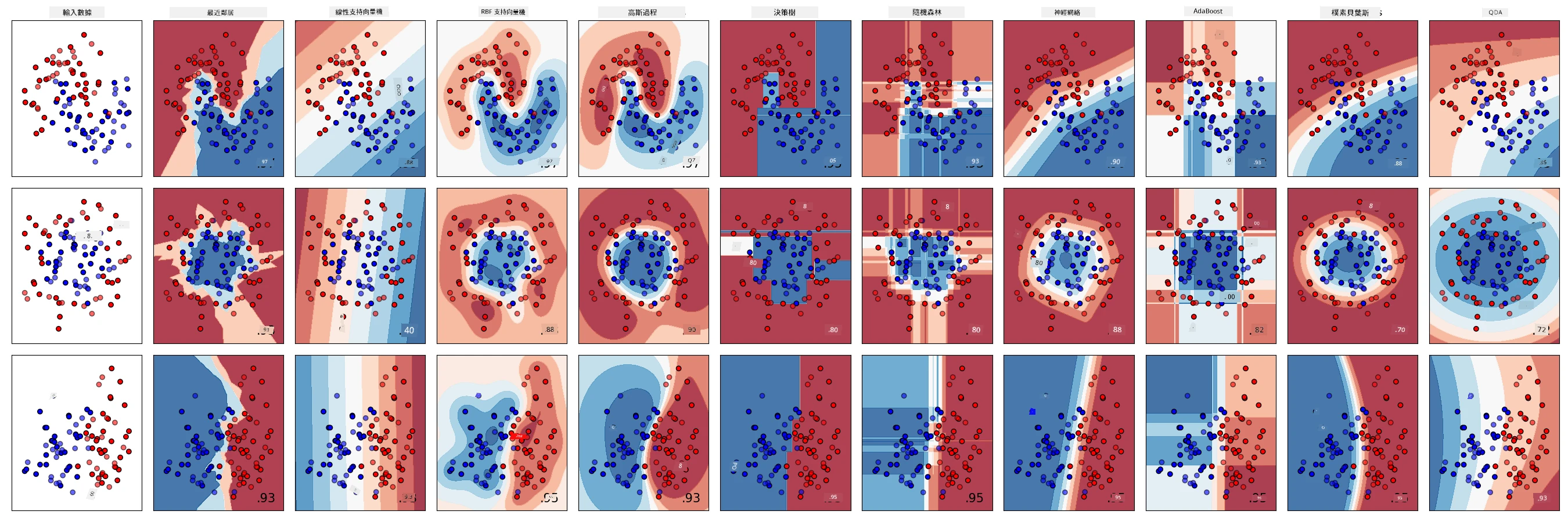
> 圖表由 Scikit-learn 文件生成
> AutoML 透過在雲端運行這些比較,輕鬆解決此問題,讓您可以選擇最適合您資料的算法。可在此[嘗試](https://docs.microsoft.com/learn/modules/automate-model-selection-with-azure-automl/?WT.mc_id=academic-77952-leestott)
### 更好的方法
比起盲目猜測,一個更好的方式是參考這份可下載的[機器學習備忘單](https://docs.microsoft.com/azure/machine-learning/algorithm-cheat-sheet?WT.mc_id=academic-77952-leestott)。這裡我們發現,對於多分類問題,我們有一些選擇:
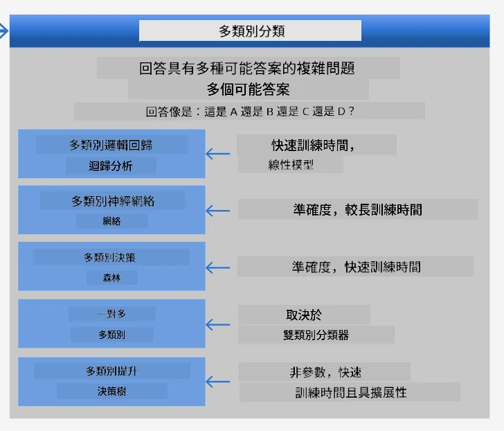
> 微軟算法備忘單的其中一部分,詳述多分類選項
✅ 下載這份備忘單,列印出來,掛在牆上!
### 推理
讓我們嘗試根據目前條件來推理不同方法:
- 神經網絡過於龐大。考慮到我們的資料清理乾淨但資料量較少,而且本地使用 notebook 進行訓練,神經網絡對此任務而言太過笨重。
- 不採用二元分類器。我們不使用二元分類器,因此排除一對多方案。
- 決策樹或邏輯回歸可能可行。決策樹可能適用,或者用於多類資料的邏輯回歸。
- 多類提升決策樹解決的問題不同。多類提升決策樹最適合非參數任務,例如設計用於建立排名的任務,因此對我們沒幫助。
### 使用 Scikit-learn
我們將使用 Scikit-learn 來分析資料。不過,在 Scikit-learn 中使用邏輯回歸的方法很多。請查看[可傳遞的參數](https://scikit-learn.org/stable/modules/generated/sklearn.linear_model.LogisticRegression.html?highlight=logistic%20regressio#sklearn.linear_model.LogisticRegression)。
本質上,我們需要指定兩個重要參數 - `multi_class` 和 `solver`,這兩個參數決定了邏輯回歸的行為。`multi_class` 值會套用某種行為,`solver` 代表要使用的演算法。並非所有 `solver` 都能與所有 `multi_class` 值搭配。
根據文件,針對多分類情況,訓練算法:
- 如果 `multi_class` 選項設為 `ovr`,**使用一對多(OvR)方案**
- 如果 `multi_class` 選項設為 `multinomial`,使用交叉熵損失。(目前 `multinomial` 選項僅由 ‘lbfgs’, ‘sag’, ‘saga’ 和 ‘newton-cg’ solver 支持)"
> 🎓 這裡的 'scheme' 可設定為 'ovr'(一對多)或 'multinomial'。由於邏輯回歸實際上是為支持二元分類設計,這些方案允許它更好地處理多分類任務。 [來源](https://machinelearningmastery.com/one-vs-rest-and-one-vs-one-for-multi-class-classification/)
> 🎓 'solver' 是指“在優化問題中要使用的算法”。[來源](https://scikit-learn.org/stable/modules/generated/sklearn.linear_model.LogisticRegression.html?highlight=logistic%20regressio#sklearn.linear_model.LogisticRegression).
Scikit-learn 提供下表說明各 solver 如何處理不同型態資料帶來的挑戰:

## 練習 - 分割資料
考慮到您最近在之前的課程已學過此內容,我們可先聚焦於邏輯回歸進行首次訓練。透過呼叫 `train_test_split()` 將資料切割為訓練集和測試集:
```python
X_train, X_test, y_train, y_test = train_test_split(cuisines_feature_df, cuisines_label_df, test_size=0.3)
```
## 練習 - 套用邏輯回歸
由於您使用的是多類情況,您需要選擇使用哪種_方案_和設定哪種_solver_。使用帶有多類設定且 solver 為 **liblinear** 的 LogisticRegression 進行訓練。
1. 創建一個多類別的邏輯回歸,將 multi_class 設為 `ovr`,solver 設為 `liblinear`:
```python
lr = LogisticRegression(multi_class='ovr',solver='liblinear')
model = lr.fit(X_train, np.ravel(y_train))
accuracy = model.score(X_test, y_test)
print ("Accuracy is {}".format(accuracy))
```
✅ 嘗試其他常用 solver,例如預設常用的 `lbfgs`
> 注意,當有需要時,使用 Pandas [`ravel`](https://pandas.pydata.org/pandas-docs/stable/reference/api/pandas.Series.ravel.html) 函數將資料攤平。
準確率相當不錯,超過 **80%**!
1. 您可以測試資料中的一列(例如 #50)以觀察模型實際表現:
```python
print(f'ingredients: {X_test.iloc[50][X_test.iloc[50]!=0].keys()}')
print(f'cuisine: {y_test.iloc[50]}')
```
結果會被印出:
```output
ingredients: Index(['cilantro', 'onion', 'pea', 'potato', 'tomato', 'vegetable_oil'], dtype='object')
cuisine: indian
```
✅ 嘗試不同列編號並檢查結果
1. 深入探索後,你可以檢查此預測的準確度:
```python
test= X_test.iloc[50].values.reshape(-1, 1).T
proba = model.predict_proba(test)
classes = model.classes_
resultdf = pd.DataFrame(data=proba, columns=classes)
topPrediction = resultdf.T.sort_values(by=[0], ascending = [False])
topPrediction.head()
```
結果輸出 - 印度菜是模型的最佳猜測,且概率很高:
| | 0 |
| -------: | -------: |
| indian | 0.715851 |
| chinese | 0.229475 |
| japanese | 0.029763 |
| korean | 0.017277 |
| thai | 0.007634 |
✅ 你能解釋為什麼模型很確定這是印度菜嗎?
1. 藉由列印分類報告取得更多細節,就像你在回歸課程中做的那樣:
```python
y_pred = model.predict(X_test)
print(classification_report(y_test,y_pred))
```
| | precision | recall | f1-score | support |
| ------------ | --------- | ------ | -------- | ------- |
| chinese | 0.73 | 0.71 | 0.72 | 229 |
| indian | 0.91 | 0.93 | 0.92 | 254 |
| japanese | 0.70 | 0.75 | 0.72 | 220 |
| korean | 0.86 | 0.76 | 0.81 | 242 |
| thai | 0.79 | 0.85 | 0.82 | 254 |
| accuracy | | | 0.80 | 1199 |
| macro avg | 0.80 | 0.80 | 0.80 | 1199 |
| weighted avg | 0.80 | 0.80 | 0.80 | 1199 |
## 🚀挑戰
在本課程中,你使用清理過的數據建立了一個機器學習模型,可以根據一系列食材預測國家料理。花點時間閱讀 Scikit-learn 提供的眾多資料分類選項。深入了解「解算器(solver)」的概念,以理解幕後運作。
## [課後測驗](https://ff-quizzes.netlify.app/en/ml/)
## 複習與自學
深入了解邏輯回歸背後的數學原理,請參閱[本課程](https://people.eecs.berkeley.edu/~russell/classes/cs194/f11/lectures/CS194%20Fall%202011%20Lecture%2006.pdf)。
## 作業
[研究解算器](assignment.md)
---
**免責聲明**:
本文件係使用 AI 翻譯服務 [Co-op Translator](https://github.com/Azure/co-op-translator) 進行翻譯。儘管我們致力於確保準確性,但請注意,機器翻譯可能包含錯誤或不準確之處。原始文件(以其母語撰寫)應視為權威來源。對於重要資訊,建議尋求專業人類翻譯。我們對因使用本翻譯而引起的任何誤解或誤釋不承擔任何責任。