# 強化学習とQ学習の紹介
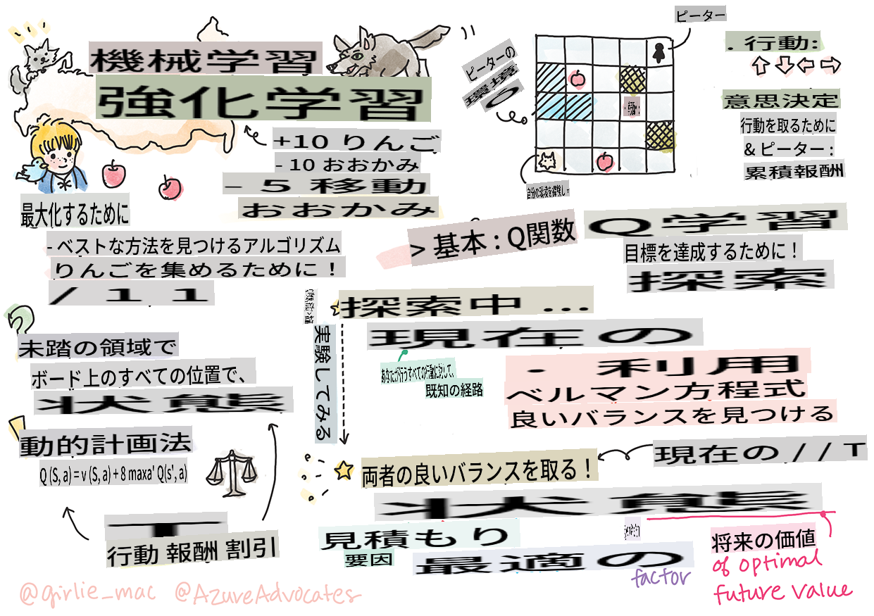
> スケッチノート: [Tomomi Imura](https://www.twitter.com/girlie_mac)
強化学習には、エージェント、状態、各状態ごとの一連のアクションという3つの重要な概念が含まれます。指定された状態でアクションを実行すると、エージェントに報酬が与えられます。コンピュータゲーム「スーパーマリオ」を想像してみてください。あなたはマリオで、崖の端に立っているゲームレベルにいます。上にはコインがあります。あなたがマリオで、特定の位置にいるゲームレベル...それがあなたの状態です。右に一歩進む(アクション)と崖から落ちてしまい、低い数値スコアが与えられます。しかし、ジャンプボタンを押すとポイントが得られ、生き残ることができます。これはポジティブな結果であり、ポジティブな数値スコアが与えられるべきです。
強化学習とシミュレーター(ゲーム)を使用することで、ゲームをプレイして報酬を最大化する方法を学ぶことができます。報酬は生き残り、できるだけ多くのポイントを獲得することです。
[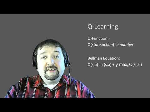](https://www.youtube.com/watch?v=lDq_en8RNOo)
> 🎥 上の画像をクリックして、Dmitry が強化学習について話すのを聞いてみましょう
## [講義前のクイズ](https://gray-sand-07a10f403.1.azurestaticapps.net/quiz/45/)
## 前提条件とセットアップ
このレッスンでは、Python でいくつかのコードを実験します。このレッスンの Jupyter Notebook コードを、自分のコンピュータ上またはクラウド上で実行できるようにしてください。
[レッスンノートブック](https://github.com/microsoft/ML-For-Beginners/blob/main/8-Reinforcement/1-QLearning/notebook.ipynb)を開いて、このレッスンを進めながら構築していくことができます。
> **Note:** クラウドからこのコードを開く場合、ノートブックコードで使用される [`rlboard.py`](https://github.com/microsoft/ML-For-Beginners/blob/main/8-Reinforcement/1-QLearning/rlboard.py) ファイルも取得する必要があります。同じディレクトリに追加してください。
## はじめに
このレッスンでは、ロシアの作曲家 [Sergei Prokofiev](https://en.wikipedia.org/wiki/Sergei_Prokofiev) による音楽童話に触発された **[ピーターと狼](https://en.wikipedia.org/wiki/Peter_and_the_Wolf)** の世界を探ります。**強化学習** を使用して、ピーターが環境を探索し、美味しいリンゴを集め、狼に出会わないようにします。
**強化学習** (RL) は、**エージェント** がいくつかの **環境** で最適な行動を学習するための技術です。エージェントはこの環境で **報酬関数** によって定義された **目標** を持つべきです。
## 環境
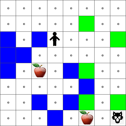
簡単にするために、ピーターの世界を次のような `width` x `height` のサイズの正方形のボードと考えます:
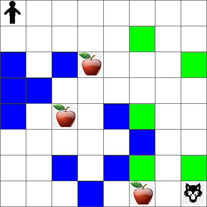
このボードの各セルは次のいずれかです:
* **地面**: ピーターや他の生き物が歩ける場所。
* **水**: 明らかに歩けない場所。
* **木** または **草**: 休む場所。
* **リンゴ**: ピーターが見つけて食べたいもの。
* **狼**: 危険で避けるべきもの。
この環境で動作するコードを含む別の Python モジュール [`rlboard.py`](https://github.com/microsoft/ML-For-Beginners/blob/main/8-Reinforcement/1-QLearning/rlboard.py) があります。このコードは概念の理解には重要ではないため、モジュールをインポートしてサンプルボードを作成します(コードブロック 1):
```python
from rlboard import *
width, height = 8,8
m = Board(width,height)
m.randomize(seed=13)
m.plot()
```
このコードは、上記の環境に似た画像を出力します。
## アクションとポリシー
この例では、ピーターの目標は狼や他の障害物を避けながらリンゴを見つけることです。これを行うために、彼はリンゴを見つけるまで基本的に歩き回ることができます。
したがって、任意の位置で、彼は次のアクションのいずれかを選択できます:上、下、左、右。
これらのアクションを辞書として定義し、それらを対応する座標の変化のペアにマッピングします。例えば、右に移動する (`R`) would correspond to a pair `(1,0)` とします(コードブロック 2):
```python
actions = { "U" : (0,-1), "D" : (0,1), "L" : (-1,0), "R" : (1,0) }
action_idx = { a : i for i,a in enumerate(actions.keys()) }
```
まとめると、このシナリオの戦略と目標は次のとおりです:
- **戦略**: エージェント(ピーター)の戦略は **ポリシー** と呼ばれる関数によって定義されます。ポリシーは任意の状態でアクションを返す関数です。私たちの場合、問題の状態はプレイヤーの現在位置を含むボードによって表されます。
- **目標**: 強化学習の目標は、問題を効率的に解決するための良いポリシーを最終的に学習することです。ただし、基準として、最も単純なポリシーである **ランダムウォーク** を考えます。
## ランダムウォーク
まず、ランダムウォーク戦略を実装して問題を解決しましょう。ランダムウォークでは、許可されたアクションから次のアクションをランダムに選択し、リンゴに到達するまで繰り返します(コードブロック 3)。
1. 以下のコードでランダムウォークを実装します:
```python
def random_policy(m):
return random.choice(list(actions))
def walk(m,policy,start_position=None):
n = 0 # number of steps
# set initial position
if start_position:
m.human = start_position
else:
m.random_start()
while True:
if m.at() == Board.Cell.apple:
return n # success!
if m.at() in [Board.Cell.wolf, Board.Cell.water]:
return -1 # eaten by wolf or drowned
while True:
a = actions[policy(m)]
new_pos = m.move_pos(m.human,a)
if m.is_valid(new_pos) and m.at(new_pos)!=Board.Cell.water:
m.move(a) # do the actual move
break
n+=1
walk(m,random_policy)
```
`walk` の呼び出しは、対応する経路の長さを返すべきです。これは実行ごとに異なる場合があります。
1. ウォーク実験を何度か(例えば100回)実行し、結果の統計を出力します(コードブロック 4):
```python
def print_statistics(policy):
s,w,n = 0,0,0
for _ in range(100):
z = walk(m,policy)
if z<0:
w+=1
else:
s += z
n += 1
print(f"Average path length = {s/n}, eaten by wolf: {w} times")
print_statistics(random_policy)
```
経路の平均長さが約30〜40ステップであることに注意してください。これは、最も近いリンゴまでの平均距離が約5〜6ステップであることを考えると、かなり多いです。
また、ランダムウォーク中のピーターの動きがどのように見えるかも確認できます:
## 報酬関数
ポリシーをより知的にするためには、どの移動が他の移動よりも「良い」かを理解する必要があります。これを行うためには、目標を定義する必要があります。
目標は、各状態に対していくつかのスコア値を返す **報酬関数** の観点から定義できます。数値が高いほど、報酬関数が良いことを意味します(コードブロック 5)。
```python
move_reward = -0.1
goal_reward = 10
end_reward = -10
def reward(m,pos=None):
pos = pos or m.human
if not m.is_valid(pos):
return end_reward
x = m.at(pos)
if x==Board.Cell.water or x == Board.Cell.wolf:
return end_reward
if x==Board.Cell.apple:
return goal_reward
return move_reward
```
報酬関数について興味深い点は、ほとんどの場合、*ゲームの最後にのみ実質的な報酬が与えられる* ことです。これは、アルゴリズムがポジティブな報酬につながる「良い」ステップを記憶し、それらの重要性を高める必要があることを意味します。同様に、悪い結果につながるすべての移動は抑制されるべきです。
## Q学習
ここで議論するアルゴリズムは **Q学習** と呼ばれます。このアルゴリズムでは、ポリシーは **Qテーブル** と呼ばれる関数(またはデータ構造)によって定義されます。これは、特定の状態で各アクションの「良さ」を記録します。
Qテーブルと呼ばれるのは、それを表形式や多次元配列として表現するのが便利なためです。ボードのサイズが `width` x `height` であるため、`width` x `height` x `len(actions)` の形状を持つ numpy 配列を使用して Qテーブルを表現できます(コードブロック 6)。
```python
Q = np.ones((width,height,len(actions)),dtype=np.float)*1.0/len(actions)
```
Qテーブルのすべての値を等しい値(この場合は 0.25)で初期化することに注意してください。これは、すべての状態でのすべての移動が等しく良いことを意味する「ランダムウォーク」ポリシーに対応します。Qテーブルを `plot` function in order to visualize the table on the board: `m.plot(Q)`.
In the center of each cell there is an "arrow" that indicates the preferred direction of movement. Since all directions are equal, a dot is displayed.
Now we need to run the simulation, explore our environment, and learn a better distribution of Q-Table values, which will allow us to find the path to the apple much faster.
## Essence of Q-Learning: Bellman Equation
Once we start moving, each action will have a corresponding reward, i.e. we can theoretically select the next action based on the highest immediate reward. However, in most states, the move will not achieve our goal of reaching the apple, and thus we cannot immediately decide which direction is better.
> Remember that it is not the immediate result that matters, but rather the final result, which we will obtain at the end of the simulation.
In order to account for this delayed reward, we need to use the principles of **[dynamic programming](https://en.wikipedia.org/wiki/Dynamic_programming)**, which allow us to think about out problem recursively.
Suppose we are now at the state *s*, and we want to move to the next state *s'*. By doing so, we will receive the immediate reward *r(s,a)*, defined by the reward function, plus some future reward. If we suppose that our Q-Table correctly reflects the "attractiveness" of each action, then at state *s'* we will chose an action *a* that corresponds to maximum value of *Q(s',a')*. Thus, the best possible future reward we could get at state *s* will be defined as `max`a'*Q(s',a')* (maximum here is computed over all possible actions *a'* at state *s'*).
This gives the **Bellman formula** for calculating the value of the Q-Table at state *s*, given action *a*:
 Here γ is the so-called **discount factor** that determines to which extent you should prefer the current reward over the future reward and vice versa.
## Learning Algorithm
Given the equation above, we can now write pseudo-code for our learning algorithm:
* Initialize Q-Table Q with equal numbers for all states and actions
* Set learning rate α ← 1
* Repeat simulation many times
1. Start at random position
1. Repeat
1. Select an action *a* at state *s*
2. Execute action by moving to a new state *s'*
3. If we encounter end-of-game condition, or total reward is too small - exit simulation
4. Compute reward *r* at the new state
5. Update Q-Function according to Bellman equation: *Q(s,a)* ← *(1-α)Q(s,a)+α(r+γ maxa'Q(s',a'))*
6. *s* ← *s'*
7. Update the total reward and decrease α.
## Exploit vs. explore
In the algorithm above, we did not specify how exactly we should choose an action at step 2.1. If we are choosing the action randomly, we will randomly **explore** the environment, and we are quite likely to die often as well as explore areas where we would not normally go. An alternative approach would be to **exploit** the Q-Table values that we already know, and thus to choose the best action (with higher Q-Table value) at state *s*. This, however, will prevent us from exploring other states, and it's likely we might not find the optimal solution.
Thus, the best approach is to strike a balance between exploration and exploitation. This can be done by choosing the action at state *s* with probabilities proportional to values in the Q-Table. In the beginning, when Q-Table values are all the same, it would correspond to a random selection, but as we learn more about our environment, we would be more likely to follow the optimal route while allowing the agent to choose the unexplored path once in a while.
## Python implementation
We are now ready to implement the learning algorithm. Before we do that, we also need some function that will convert arbitrary numbers in the Q-Table into a vector of probabilities for corresponding actions.
1. Create a function `probs()` に渡すことができます:
```python
def probs(v,eps=1e-4):
v = v-v.min()+eps
v = v/v.sum()
return v
```
初期状態でベクトルのすべての成分が同一である場合に 0 で割ることを避けるために、元のベクトルにいくつかの `eps` を追加します。
5000回の実験(エポック)を通じて学習アルゴリズムを実行します(コードブロック 8)。
```python
for epoch in range(5000):
# Pick initial point
m.random_start()
# Start travelling
n=0
cum_reward = 0
while True:
x,y = m.human
v = probs(Q[x,y])
a = random.choices(list(actions),weights=v)[0]
dpos = actions[a]
m.move(dpos,check_correctness=False) # we allow player to move outside the board, which terminates episode
r = reward(m)
cum_reward += r
if r==end_reward or cum_reward < -1000:
lpath.append(n)
break
alpha = np.exp(-n / 10e5)
gamma = 0.5
ai = action_idx[a]
Q[x,y,ai] = (1 - alpha) * Q[x,y,ai] + alpha * (r + gamma * Q[x+dpos[0], y+dpos[1]].max())
n+=1
```
このアルゴリズムを実行した後、Qテーブルは各ステップでの異なるアクションの魅力を定義する値で更新されます。Qテーブルを視覚化して、各セルに小さな円を描くことで、移動の希望方向を示すベクトルをプロットすることができます。
## ポリシーの確認
Qテーブルは各状態での各アクションの「魅力」をリストしているため、効率的なナビゲーションを定義するのに簡単に使用できます。最も簡単な場合、Qテーブルの値が最も高いアクションを選択できます(コードブロック 9)。
```python
def qpolicy_strict(m):
x,y = m.human
v = probs(Q[x,y])
a = list(actions)[np.argmax(v)]
return a
walk(m,qpolicy_strict)
```
> 上記のコードを数回試してみると、時々「ハング」することがあり、ノートブックの STOP ボタンを押して中断する必要があることに気付くかもしれません。これは、最適な Q値の観点から2つの状態が互いに「指し示す」状況があり、その場合、エージェントが無限にその状態間を移動し続けるためです。
## 🚀チャレンジ
> **タスク 1:** `walk` function to limit the maximum length of path by a certain number of steps (say, 100), and watch the code above return this value from time to time.
> **Task 2:** Modify the `walk` function so that it does not go back to the places where it has already been previously. This will prevent `walk` from looping, however, the agent can still end up being "trapped" in a location from which it is unable to escape.
## Navigation
A better navigation policy would be the one that we used during training, which combines exploitation and exploration. In this policy, we will select each action with a certain probability, proportional to the values in the Q-Table. This strategy may still result in the agent returning back to a position it has already explored, but, as you can see from the code below, it results in a very short average path to the desired location (remember that `print_statistics` を修正して、シミュレーションを100回実行します(コードブロック 10)。
```python
def qpolicy(m):
x,y = m.human
v = probs(Q[x,y])
a = random.choices(list(actions),weights=v)[0]
return a
print_statistics(qpolicy)
```
このコードを実行した後、以前よりも平均経路長がはるかに短くなり、3〜6の範囲になります。
## 学習プロセスの調査
学習プロセスは、問題空間の構造に関する獲得した知識の探索と探索のバランスです。学習の結果(エージェントが目標に到達するための短い経路を見つける能力)が向上したことがわかりましたが、学習プロセス中の平均経路長の変化を観察することも興味深いです。
学習の要点をまとめると:
- **平均経路長の増加**。最初は平均経路長が増加します。これは、環境について何も知らないときに、悪い状態(水や狼)に閉じ込められやすいことが原因です。より多くを学び、この知識を使い始めると、環境をより長く探索できますが、リンゴの位置についてはまだよくわかりません。
- **学習が進むにつれて経路長が減少**。十分に学習すると、エージェントが目標を達成するのが簡単になり、経路長が減少し始めます。ただし、探索は続けているため、最適な経路から逸れ、新しいオプションを探索することがあり、経路が最適より長くなることがあります。
- **突然の経路長の増加**。グラフで経路長が突然増加することもあります。これはプロセスの確率的な性質を示しており、新しい値で Qテーブルの係数を上書きすることで Qテーブルが「損なわれる」可能性があります。理想的には、学習率を低下させることでこれを最小限に抑えるべきです(例えば、学習の終わりに向かって、Qテーブルの値をわずかに調整する)。
全体として、学習プロセスの成功と質は、学習率、学習率の減衰、割引率などのパラメータに大きく依存することを覚えておくことが重要です。これらは **ハイパーパラメータ** と呼ばれ、**パラメータ** とは区別されます。パラメータは学習中に最適化するものであり(例えば、Qテーブルの係数)、最適なハイパーパラメータ値を見つけるプロセスは **ハイパーパラメータ最適化** と呼ばれ、別のトピックとして取り上げる価値があります。
## [講義後のクイズ](https://gray-sand-07a10f403.1.azurestaticapps.net/quiz/46/)
## 課題
[より現実的な世界](assignment.md)
**免責事項**:
この文書は機械翻訳AIサービスを使用して翻訳されています。正確さを期していますが、自動翻訳には誤りや不正確さが含まれる場合がありますのでご注意ください。元の言語で記載された文書が信頼できる情報源と見なされるべきです。重要な情報については、専門の人間による翻訳をお勧めします。この翻訳の使用に起因する誤解や誤った解釈について、当社は一切の責任を負いません。
Here γ is the so-called **discount factor** that determines to which extent you should prefer the current reward over the future reward and vice versa.
## Learning Algorithm
Given the equation above, we can now write pseudo-code for our learning algorithm:
* Initialize Q-Table Q with equal numbers for all states and actions
* Set learning rate α ← 1
* Repeat simulation many times
1. Start at random position
1. Repeat
1. Select an action *a* at state *s*
2. Execute action by moving to a new state *s'*
3. If we encounter end-of-game condition, or total reward is too small - exit simulation
4. Compute reward *r* at the new state
5. Update Q-Function according to Bellman equation: *Q(s,a)* ← *(1-α)Q(s,a)+α(r+γ maxa'Q(s',a'))*
6. *s* ← *s'*
7. Update the total reward and decrease α.
## Exploit vs. explore
In the algorithm above, we did not specify how exactly we should choose an action at step 2.1. If we are choosing the action randomly, we will randomly **explore** the environment, and we are quite likely to die often as well as explore areas where we would not normally go. An alternative approach would be to **exploit** the Q-Table values that we already know, and thus to choose the best action (with higher Q-Table value) at state *s*. This, however, will prevent us from exploring other states, and it's likely we might not find the optimal solution.
Thus, the best approach is to strike a balance between exploration and exploitation. This can be done by choosing the action at state *s* with probabilities proportional to values in the Q-Table. In the beginning, when Q-Table values are all the same, it would correspond to a random selection, but as we learn more about our environment, we would be more likely to follow the optimal route while allowing the agent to choose the unexplored path once in a while.
## Python implementation
We are now ready to implement the learning algorithm. Before we do that, we also need some function that will convert arbitrary numbers in the Q-Table into a vector of probabilities for corresponding actions.
1. Create a function `probs()` に渡すことができます:
```python
def probs(v,eps=1e-4):
v = v-v.min()+eps
v = v/v.sum()
return v
```
初期状態でベクトルのすべての成分が同一である場合に 0 で割ることを避けるために、元のベクトルにいくつかの `eps` を追加します。
5000回の実験(エポック)を通じて学習アルゴリズムを実行します(コードブロック 8)。
```python
for epoch in range(5000):
# Pick initial point
m.random_start()
# Start travelling
n=0
cum_reward = 0
while True:
x,y = m.human
v = probs(Q[x,y])
a = random.choices(list(actions),weights=v)[0]
dpos = actions[a]
m.move(dpos,check_correctness=False) # we allow player to move outside the board, which terminates episode
r = reward(m)
cum_reward += r
if r==end_reward or cum_reward < -1000:
lpath.append(n)
break
alpha = np.exp(-n / 10e5)
gamma = 0.5
ai = action_idx[a]
Q[x,y,ai] = (1 - alpha) * Q[x,y,ai] + alpha * (r + gamma * Q[x+dpos[0], y+dpos[1]].max())
n+=1
```
このアルゴリズムを実行した後、Qテーブルは各ステップでの異なるアクションの魅力を定義する値で更新されます。Qテーブルを視覚化して、各セルに小さな円を描くことで、移動の希望方向を示すベクトルをプロットすることができます。
## ポリシーの確認
Qテーブルは各状態での各アクションの「魅力」をリストしているため、効率的なナビゲーションを定義するのに簡単に使用できます。最も簡単な場合、Qテーブルの値が最も高いアクションを選択できます(コードブロック 9)。
```python
def qpolicy_strict(m):
x,y = m.human
v = probs(Q[x,y])
a = list(actions)[np.argmax(v)]
return a
walk(m,qpolicy_strict)
```
> 上記のコードを数回試してみると、時々「ハング」することがあり、ノートブックの STOP ボタンを押して中断する必要があることに気付くかもしれません。これは、最適な Q値の観点から2つの状態が互いに「指し示す」状況があり、その場合、エージェントが無限にその状態間を移動し続けるためです。
## 🚀チャレンジ
> **タスク 1:** `walk` function to limit the maximum length of path by a certain number of steps (say, 100), and watch the code above return this value from time to time.
> **Task 2:** Modify the `walk` function so that it does not go back to the places where it has already been previously. This will prevent `walk` from looping, however, the agent can still end up being "trapped" in a location from which it is unable to escape.
## Navigation
A better navigation policy would be the one that we used during training, which combines exploitation and exploration. In this policy, we will select each action with a certain probability, proportional to the values in the Q-Table. This strategy may still result in the agent returning back to a position it has already explored, but, as you can see from the code below, it results in a very short average path to the desired location (remember that `print_statistics` を修正して、シミュレーションを100回実行します(コードブロック 10)。
```python
def qpolicy(m):
x,y = m.human
v = probs(Q[x,y])
a = random.choices(list(actions),weights=v)[0]
return a
print_statistics(qpolicy)
```
このコードを実行した後、以前よりも平均経路長がはるかに短くなり、3〜6の範囲になります。
## 学習プロセスの調査
学習プロセスは、問題空間の構造に関する獲得した知識の探索と探索のバランスです。学習の結果(エージェントが目標に到達するための短い経路を見つける能力)が向上したことがわかりましたが、学習プロセス中の平均経路長の変化を観察することも興味深いです。
学習の要点をまとめると:
- **平均経路長の増加**。最初は平均経路長が増加します。これは、環境について何も知らないときに、悪い状態(水や狼)に閉じ込められやすいことが原因です。より多くを学び、この知識を使い始めると、環境をより長く探索できますが、リンゴの位置についてはまだよくわかりません。
- **学習が進むにつれて経路長が減少**。十分に学習すると、エージェントが目標を達成するのが簡単になり、経路長が減少し始めます。ただし、探索は続けているため、最適な経路から逸れ、新しいオプションを探索することがあり、経路が最適より長くなることがあります。
- **突然の経路長の増加**。グラフで経路長が突然増加することもあります。これはプロセスの確率的な性質を示しており、新しい値で Qテーブルの係数を上書きすることで Qテーブルが「損なわれる」可能性があります。理想的には、学習率を低下させることでこれを最小限に抑えるべきです(例えば、学習の終わりに向かって、Qテーブルの値をわずかに調整する)。
全体として、学習プロセスの成功と質は、学習率、学習率の減衰、割引率などのパラメータに大きく依存することを覚えておくことが重要です。これらは **ハイパーパラメータ** と呼ばれ、**パラメータ** とは区別されます。パラメータは学習中に最適化するものであり(例えば、Qテーブルの係数)、最適なハイパーパラメータ値を見つけるプロセスは **ハイパーパラメータ最適化** と呼ばれ、別のトピックとして取り上げる価値があります。
## [講義後のクイズ](https://gray-sand-07a10f403.1.azurestaticapps.net/quiz/46/)
## 課題
[より現実的な世界](assignment.md)
**免責事項**:
この文書は機械翻訳AIサービスを使用して翻訳されています。正確さを期していますが、自動翻訳には誤りや不正確さが含まれる場合がありますのでご注意ください。元の言語で記載された文書が信頼できる情報源と見なされるべきです。重要な情報については、専門の人間による翻訳をお勧めします。この翻訳の使用に起因する誤解や誤った解釈について、当社は一切の責任を負いません。