|
|
2 weeks ago | |
|---|---|---|
| .. | ||
| solution | 3 weeks ago | |
| README.md | 2 weeks ago | |
| assignment.md | 3 weeks ago | |
| notebook.ipynb | 3 weeks ago | |
README.md
အချိုးအစားများကိုမြင်သာအောင်ဖော်ပြခြင်း
 |
|---|
| အချိုးအစားများကိုမြင်သာအောင်ဖော်ပြခြင်း - Sketchnote by @nitya |
ဒီသင်ခန်းစာမှာ သင်သည် သဘာဝနှင့်ဆက်စပ်သောအခြား dataset ကိုအသုံးပြုပြီး အချိုးအစားများကိုမြင်သာအောင်ဖော်ပြပါမည်။ ဥပမာအားဖြင့် မုန့်ဖုတ် dataset တွင် မုန့်ဖုတ်အမျိုးအစားများ ဘယ်လောက်ရှိသည်ကိုဖော်ပြပါမည်။ Audubon မှရရှိသော Agaricus နှင့် Lepiota မိသားစုများတွင်ပါဝင်သော gilled မုန့်ဖုတ် 23 မျိုးအကြောင်းအချက်အလက်များကို အသုံးပြု၍ မုန့်ဖုတ်များကို စူးစမ်းလေ့လာကြမည်။ သင်သည် အောက်ပါအချိုးအစားများကိုဖော်ပြနိုင်သောအမျိုးအစားများကို စမ်းသပ်နိုင်ပါမည်-
- ပိုင်း chart 🥧
- ဒိုနတ် chart 🍩
- ဝါဖယ် chart 🧇
💡 Microsoft Research မှ Charticulator ဆိုသော စိတ်ဝင်စားဖွယ်ကောင်းသော project တစ်ခုသည် data visualizations အတွက် drag and drop interface ကို အခမဲ့ပေးထားသည်။ သူတို့၏ tutorial တစ်ခုတွင်လည်း ဒီမုန့်ဖုတ် dataset ကိုအသုံးပြုထားသည်! ဒါကြောင့် သင် dataset ကိုလေ့လာပြီး library ကိုတစ်ချိန်တည်းမှာလည်းသင်ယူနိုင်သည်။ Charticulator tutorial ကိုကြည့်ပါ။
Pre-lecture quiz
မုန့်ဖုတ်များကိုလေ့လာကြမယ် 🍄
မုန့်ဖုတ်များသည် အလွန်စိတ်ဝင်စားဖွယ်ကောင်းသည်။ dataset ကို import လုပ်ပြီး လေ့လာကြမယ်-
import pandas as pd
import matplotlib.pyplot as plt
mushrooms = pd.read_csv('../../data/mushrooms.csv')
mushrooms.head()
အချက်အလက်များကိုလေ့လာရန်အတွက် အလွန်ကောင်းသော table တစ်ခု print ထုတ်ထားသည်-
| class | cap-shape | cap-surface | cap-color | bruises | odor | gill-attachment | gill-spacing | gill-size | gill-color | stalk-shape | stalk-root | stalk-surface-above-ring | stalk-surface-below-ring | stalk-color-above-ring | stalk-color-below-ring | veil-type | veil-color | ring-number | ring-type | spore-print-color | population | habitat |
|---|---|---|---|---|---|---|---|---|---|---|---|---|---|---|---|---|---|---|---|---|---|---|
| Poisonous | Convex | Smooth | Brown | Bruises | Pungent | Free | Close | Narrow | Black | Enlarging | Equal | Smooth | Smooth | White | White | Partial | White | One | Pendant | Black | Scattered | Urban |
| Edible | Convex | Smooth | Yellow | Bruises | Almond | Free | Close | Broad | Black | Enlarging | Club | Smooth | Smooth | White | White | Partial | White | One | Pendant | Brown | Numerous | Grasses |
| Edible | Bell | Smooth | White | Bruises | Anise | Free | Close | Broad | Brown | Enlarging | Club | Smooth | Smooth | White | White | Partial | White | One | Pendant | Brown | Numerous | Meadows |
| Poisonous | Convex | Scaly | White | Bruises | Pungent | Free | Close | Narrow | Brown | Enlarging | Equal | Smooth | Smooth | White | White | Partial | White | One | Pendant | Black | Scattered | Urban |
အချက်အလက်များသည် text အဖြစ်ရှိနေသည်ကို သင်ချက်ချင်းသတိပြုမိပါသည်။ chart တွင်အသုံးပြုနိုင်ရန်အတွက် data ကိုပြောင်းလဲရန်လိုအပ်ပါသည်။ အချက်အလက်များသည် object အဖြစ်ကိုယ်စားပြုထားသည်-
print(mushrooms.select_dtypes(["object"]).columns)
output သည်-
Index(['class', 'cap-shape', 'cap-surface', 'cap-color', 'bruises', 'odor',
       'gill-attachment', 'gill-spacing', 'gill-size', 'gill-color',
       'stalk-shape', 'stalk-root', 'stalk-surface-above-ring',
       'stalk-surface-below-ring', 'stalk-color-above-ring',
       'stalk-color-below-ring', 'veil-type', 'veil-color', 'ring-number',
       'ring-type', 'spore-print-color', 'population', 'habitat'],
      dtype='object')
ဒီ data ကိုယူပြီး 'class' column ကို category အဖြစ်ပြောင်းပါ-
cols = mushrooms.select_dtypes(["object"]).columns
mushrooms[cols] = mushrooms[cols].astype('category')
edibleclass=mushrooms.groupby(['class']).count()
edibleclass
အခု သင်မုန့်ဖုတ် data ကို print ထုတ်ပါက poisonous/edible class အလိုက် category အဖြစ် grouped ဖြစ်နေသည်ကိုမြင်နိုင်ပါသည်-
| cap-shape | cap-surface | cap-color | bruises | odor | gill-attachment | gill-spacing | gill-size | gill-color | stalk-shape | ... | stalk-surface-below-ring | stalk-color-above-ring | stalk-color-below-ring | veil-type | veil-color | ring-number | ring-type | spore-print-color | population | habitat | |
|---|---|---|---|---|---|---|---|---|---|---|---|---|---|---|---|---|---|---|---|---|---|
| class | |||||||||||||||||||||
| Edible | 4208 | 4208 | 4208 | 4208 | 4208 | 4208 | 4208 | 4208 | 4208 | 4208 | ... | 4208 | 4208 | 4208 | 4208 | 4208 | 4208 | 4208 | 4208 | 4208 | 4208 |
| Poisonous | 3916 | 3916 | 3916 | 3916 | 3916 | 3916 | 3916 | 3916 | 3916 | 3916 | ... | 3916 | 3916 | 3916 | 3916 | 3916 | 3916 | 3916 | 3916 | 3916 | 3916 |
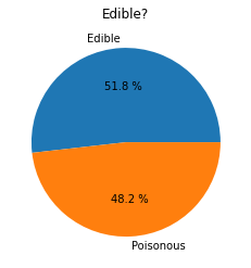
ဒီ table တွင်ဖော်ပြထားသော အစီအစဉ်အတိုင်း class category labels များကိုဖန်တီးပါက pie chart တစ်ခုကိုဖန်တီးနိုင်ပါသည်-
Pie!
labels=['Edible','Poisonous']
plt.pie(edibleclass['population'],labels=labels,autopct='%.1f %%')
plt.title('Edible?')
plt.show()
Voila, ဒီ data ကို poisonous/edible class နှစ်ခုအလိုက် အချိုးအစားများကိုဖော်ပြထားသော pie chart တစ်ခုဖြစ်သည်။ label array ကိုဖန်တီးရာတွင် label အစီအစဉ်ကိုမှန်ကန်စေရန် verify လုပ်ရန်အရေးကြီးသည်။
Donuts!
ပိုမိုစိတ်ဝင်စားဖွယ်ကောင်းသော pie chart တစ်ခုမှာ donut chart ဖြစ်ပြီး pie chart ၏အလယ်တွင်အပေါက်ရှိသည်။ ဒီနည်းလမ်းကိုအသုံးပြုပြီး data ကိုကြည့်ပါ။
မုန့်ဖုတ်များပေါက်နေသောနေရာများကိုကြည့်ပါ-
habitat=mushrooms.groupby(['habitat']).count()
habitat
ဒီမှာ သင်သည် data ကို habitat အလိုက် grouped လုပ်ထားသည်။ 7 ခုရှိပြီး donut chart အတွက် labels အဖြစ်အသုံးပြုပါ-
labels=['Grasses','Leaves','Meadows','Paths','Urban','Waste','Wood']

plt.pie(habitat['class'], labels=labels,
        autopct='%1.1f%%', pctdistance=0.85)

center_circle = plt.Circle((0, 0), 0.40, fc='white')
fig = plt.gcf()

fig.gca().add_artist(center_circle)

plt.title('Mushroom Habitats')

plt.show()
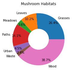
ဒီ code သည် chart တစ်ခုနှင့် center circle တစ်ခုကိုဆွဲပြီး ထို့နောက် center circle ကို chart တွင်ထည့်သည်။ center circle ၏ width ကို 0.40 ကိုအခြားတန်ဖိုးဖြင့်ပြောင်းလဲခြင်းဖြင့် edit လုပ်နိုင်သည်။
Donut charts များကို labels များကိုထင်ရှားစေရန်အမျိုးမျိုးပြောင်းလဲနိုင်သည်။ docs တွင်ပိုမိုလေ့လာပါ။
အခု သင်သည် data ကို grouped လုပ်ပြီး pie သို့မဟုတ် donut အဖြစ်ဖော်ပြနိုင်သည်။ အခြား chart အမျိုးအစားများကိုလည်းစမ်းသပ်ကြည့်ပါ။ ဝါဖယ် chart ကိုစမ်းကြည့်ပါ၊ ဒါဟာ quantity ကိုတစ်ခြားနည်းလမ်းဖြင့်ဖော်ပြခြင်းဖြစ်သည်။
Waffles!
'Waffle' type chart သည် quantity များကို 2D array of squares အဖြစ်ဖော်ပြသောနည်းလမ်းတစ်ခုဖြစ်သည်။ dataset တွင် မုန့်ဖုတ် cap color များ၏ quantity များကိုဖော်ပြရန်စမ်းကြည့်ပါ။ ဒီအတွက် PyWaffle ဆိုသော helper library ကို install လုပ်ပြီး Matplotlib ကိုအသုံးပြုပါ-
pip install pywaffle
data segment တစ်ခုကိုရွေးပါ-
capcolor=mushrooms.groupby(['cap-color']).count()
capcolor
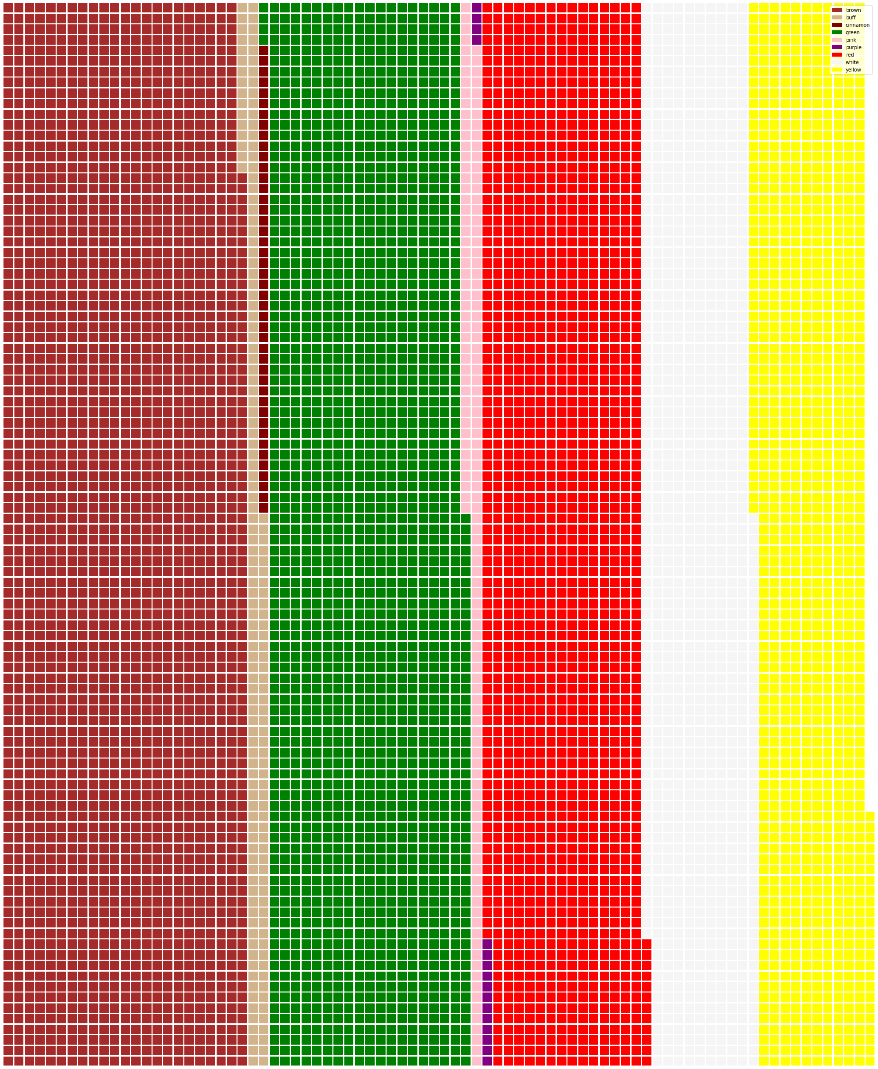
labels များဖန်တီးပြီး data ကို grouped လုပ်ကာ waffle chart တစ်ခုဖန်တီးပါ-
import pandas as pd
import matplotlib.pyplot as plt
from pywaffle import Waffle

data ={'color': ['brown', 'buff', 'cinnamon', 'green', 'pink', 'purple', 'red', 'white', 'yellow'],
    'amount': capcolor['class']
     }

df = pd.DataFrame(data)

fig = plt.figure(
    FigureClass = Waffle,
    rows = 100,
    values = df.amount,
    labels = list(df.color),
    figsize = (30,30),
    colors=["brown", "tan", "maroon", "green", "pink", "purple", "red", "whitesmoke", "yellow"],
)
Waffle chart ကိုအသုံးပြု၍ dataset တွင် မုန့်ဖုတ် cap color များ၏အချိုးအစားများကိုရှင်းလင်းစွာမြင်နိုင်သည်။ စိတ်ဝင်စားစရာကောင်းသည်မှာ အစိမ်းရောင် cap မုန့်ဖုတ်များစွာရှိနေသည်။
✅ Pywaffle သည် Font Awesome တွင်ရရှိနိုင်သော icon များကို chart တွင်ထည့်သွင်းနိုင်သည်။ square များအစား icon များကိုအသုံးပြု၍ ပိုမိုစိတ်ဝင်စားဖွယ်ကောင်းသော waffle chart ကိုဖန်တီးရန်စမ်းကြည့်ပါ။
ဒီသင်ခန်းစာတွင် သင်သည် အချိုးအစားများကိုဖော်ပြရန်နည်းလမ်း ၃ မျိုးကိုသင်ယူခဲ့သည်။ ပထမဦးဆုံး data ကို category များအလိုက် grouped လုပ်ပြီး data ကိုဖော်ပြရန်အကောင်းဆုံးနည်းလမ်းကိုဆုံးဖြတ်ပါ - pie, donut, သို့မဟုတ် waffle။ အားလုံးသည် user ကို dataset ၏ snapshot တစ်ခုကိုချက်ချင်းမြင်နိုင်စေသည်။
🚀 စိန်ခေါ်မှု
ဒီအချိုးအစားများကို Charticulator တွင်ပြန်ဖန်တီးကြည့်ပါ။
Post-lecture quiz
ပြန်လည်သုံးသပ်ခြင်းနှင့် ကိုယ်တိုင်လေ့လာခြင်း
Pie, donut, သို့မဟုတ် waffle chart ကိုဘယ်အချိန်မှာအသုံးပြုရမယ်ဆိုတာမရှင်းလင်းနိုင်တဲ့အခါတွေရှိတတ်သည်။ ဒီအကြောင်းအရာကိုဖတ်ရှုရန်အောက်ပါဆောင်းပါးများကိုကြည့်ပါ-
https://www.beautiful.ai/blog/battle-of-the-charts-pie-chart-vs-donut-chart
https://medium.com/@hypsypops/pie-chart-vs-donut-chart-showdown-in-the-ring-5d24fd86a9ce
https://www.mit.edu/~mbarker/formula1/f1help/11-ch-c6.htm
Pie, donut, waffle chart များကိုရွေးချယ်ရန်ပိုမိုသိရှိရန် သုတေသနလုပ်ပါ။
လုပ်ငန်းတာဝန်
အကြောင်းကြားချက်:
ဤစာရွက်စာတမ်းကို AI ဘာသာပြန်ဝန်ဆောင်မှု Co-op Translator ကို အသုံးပြု၍ ဘာသာပြန်ထားပါသည်။ ကျွန်ုပ်တို့သည် တိကျမှုအတွက် ကြိုးစားနေသော်လည်း၊ အလိုအလျောက် ဘာသာပြန်ခြင်းတွင် အမှားများ သို့မဟုတ် မမှန်ကန်မှုများ ပါဝင်နိုင်သည်ကို သတိပြုပါ။ မူရင်းဘာသာစကားဖြင့် ရေးသားထားသော စာရွက်စာတမ်းကို အာဏာတရ အရင်းအမြစ်အဖြစ် ရှုလေ့လာသင့်ပါသည်။ အရေးကြီးသော အချက်အလက်များအတွက် လူ့ဘာသာပြန်ပညာရှင်များမှ ပရော်ဖက်ရှင်နယ် ဘာသာပြန်ခြင်းကို အကြံပြုပါသည်။ ဤဘာသာပြန်ကို အသုံးပြုခြင်းမှ ဖြစ်ပေါ်လာသော အလွဲအလွတ်များ သို့မဟုတ် အနားယူမှားမှုများအတွက် ကျွန်ုပ်တို့သည် တာဝန်မယူပါ။